
|
|
|
Bioluminescent imaging has the capability to reveal molecular and cellular activities directly, and can be applied to all disease processes in most small-animal models. It is very sensitive, and helps diagnose diseases, monitor therapies, and facilitate drug development.1, 2 Bioluminescent imaging has been in a planar mode and largely a qualitative imaging tool.3 With bioluminescence tomography (BLT), 3-D localization and quantification is enabled of a bioluminescence source distribution inside a living small animal such as a mouse.4, 5 In bioluminescence imaging, photon scattering predominates over absorption in the biological tissue in this spectral range of interest. As a result, a significant number of bioluminescent photons can escape the attenuating environment, and they can be detected using a highly sensitive charge-coupled device (CCD) camera.3 In this case, the photons propagation in the biological tissue can be well described by steady-state diffusion equation and Robin-type boundary conditions.6, 7 The BLT principles and solution uniqueness for the BLT problem conditions were studied under some practical conditions. 4, 5, 8, 9 Some numerical algorithms for BLT were already reported, including the finite element based BLT algorithms, 10, 11, 12, 13, 14 BLT in combination with PET (OPET),15 multispectral bioluminescence optical tomography,16, 17 and BLT method based on diffusion theory of half infinite medium.18 In this letter, for the first time we develop a BLT algorithm using the boundary integral method. This methodology only requires finite element meshing of structural boundaries instead of complex volumetric finite elements previously used for BLT. Hence, the complexity and stability of the new BLT algorithm are improved as compared to that of the finite-element-based BLT algorithms. The overall support region of a small animal can be decomposed into a number of subregions with ; for example, lungs, heart, liver, bone, muscle, and so on. Applying the Gauss theorem, the steady-state diffusion equation can be transformed to a boundary integral equation on each subregion19: where is a Green function of the steady-state diffusion equation, is the diffusion coefficient given by , and where is the absorption coefficient and is the reduced scattering coefficient for the subregion . Equation 1 is a well-posed second kind integral equation. The bounding surface can then be split into surface elements on which the function and are approximated by use of a set of interpolation points and interpolation functions on 19:The shape of the surface element can be arbitrarily selected, and usually made as a quadrilateral or a triangle. The number of points per surface element depends on the accuracy needed in the interpolation procedure. Let and represent the values of the function and at an interpolation point , respectively. Since the BLT reconstruction is underdetermined and ill-posed, we incorporate a priori knowledge to define a permissible source region for a subregion without loss of generality, where the bioluminescence source may be distributed. The region can be discretized, and the embedded source function is approximated on aswhere represent the value of the source function at an interpolation point is the interpolation basis function, and is the number of discrete values of the source function.Inserting Eqs. 2, 3 into Eq. 1, we obtain the following matrix equation: where , , is the number of nodal points for , , and is a strictly diagonally dominant matrix, and allows its inversion. Multiplying Eq. 4 with the inverse , we haveFurthermore, in terms of the continuity of and at the interface and the Robin-type external boundary condition, the above matrix equation for can be assembled into19 where denotes the source distribution in the permissible source region, and a vector consisting of photon density values at the boundary and interface nodes, which can be divided into at internal interface nodes and at exterior boundary nodes. Because is still a diagonally dominant matrix and invertible, we have . After removal of those rows of that correspond to we obtain and a linear relationship between measurable photon density at boundary nodes and the source distributionGenerally, the measured data in bioluminescence imaging are corrupted by noise, so it is not practical to solve for directly from Eq.7. Instead, an optimization procedure is employed to find a solution by minimizing the following objective function:where is the upper bound that is chosen to be physically meaningful, a stabilizing function, the regularization parameter, the weight matrix, and .To demonstrate the feasibility and efficiency of our new algorithm, we carried out an experiment using a heterogeneous mouse chest phantom. The physical phantom of 30-mm height and 30-mm diameter was fabricated. It consisted of four types of high-density polyethylene materials: (8624K16), nylon 6/6 (8538K23), delrin (8579K21), and polypropylene (8658K11) (McMaster-Carr Supply Company, Chicago, Illinois), to represent muscle (M), lungs (L), heart (H), and bone (B) respectively. Based on the diffuse model of photon propagation, the optical parameters of the four materials at wavelength of about were independently found from transillumination experimental data,12 which are listed in Table 1 . The luminescent light stick (Glowproducts, Victoria, British Columbia, Canada) was selected as the testing source. The stick consisted of a small glass vial containing one chemical solution and a large plastic vial containing another solution, with the former being embedded in the latter. By bending the plastic vial, the glass vial can be broken to mix the two solutions and emit red light around , which is spectrally similar to bioluminescent light generated by the luciferase. Two small holes of diameter and height were longitudinally drilled in the left lung region of the phantom with their centers at and , respectively, as shown in Fig. 1 . Two catheter tubes about in height were filled with red luminescent liquid, and were placed inside the two holes as light sources, respectively. Emitting light power of two catheter tubes was measured with the CCD camera. They were 105.1 nW and , respectively. Fig. 1Heterogeneous mouse chest phantom. (a) A geometrical model of the phantom embedded with two sources; (b) a middle cross-section through two embedded hollow cylinders for hosting luminescent sources in one lung.  Table 1Optical parameters of the heterogeneous mouse chest phantom.
The experiment was conducted in a totally dark environment to avoid background noise. The flux density on the cylindrical surface of the phantom was recorded with the sensitive CCD camera, along four radial directions separated by , as schematically shown in Fig. 1b. During each data acquisition session, one luminescent view was taken by exposing the camera for , as shown in Fig. 2 Fig. 2Luminescent views of the side surface of the cylindrical phantom taken using a CCD camera in four directions of apart, (a)–(d) Front, back, left, and right views, respectively.  A permissible source region was assigned as to regularize the BLT solution. Along the longitudinal direction high signal-to-noise ratios (SNR) were clustered between to relative to the phantom bottom. Beyond the above region, the SNR were insignificant, and ignored to reduce the computational cost. To simulate the photon propagation in the phantom, a geometrical model of diameter and height was constructed corresponding to a middle section of the physical phantom. Based on this model, a discrete mesh was generated for the external boundary and internal interface. The external boundary mesh consisted of 960 quadrilateral elements and 1024 measurement datum points. The internal interface mesh consisted of 1680 quadrilateral elements and 1792 nodes. The permissible source region was also discretized into 308 wedge elements, as shown in Fig. 3b. The measured photon density at each detector location was computed from the CCD luminescent image using our calibration formula. Then, the proposed algorithm was applied to reconstruct the light source distribution in the heterogeneous phantom. The reconstructed results correctly revealed that there were two strong light sources in the phantom located at with flux density and at with , respectively. The former was estimated to yield a total power of (the total flux , while the latter was computed to have a total power of . Figures 3a and 3b shows the reconstructed source distribution. The differences between the reconstructed and real source positions were 1.9 and for the two sources, respectively. The relative errors in the source strength were 3.0% and 15.3%, respectively. The computed surface photon density profiles based on the reconstructed light sources were in good agreement with the experimental counterparts with an average relative error about 20%. Fig. 3BLT reconstruction of the mouse chest phantom. (a) The 3-D and (b) the 2-D reconstructed source distribution in the permissible region. 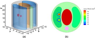 In conclusion, we have developed a boundary integral method to reconstruct a 3-D bioluminescent source distribution embedded in a heterogeneous object of interest from measured flux data on the external surface of the object. The feasibility of the new reconstruction method has been demonstrated in a physical heterogeneous phantom experiment. The results have indicated that the method can reliably localize the source locations, and recover the source strength fairly well. The reconstruction results may be further improved by decreasing the boundary element size, lowering the measurement noise, and increasing the accuracy of optical parameters. The method only requires the discretization on the object boundary and structural interface, which is much easier than meshing for volumetric finite elements. Hence, the new method can handle a complex geometrical model much efficiently than finite element based BLT algorithm. AcknowledgementsThis work is supported by an NIH/NIBIB Grant EB001685 and the U.S. Army's Breast Cancer Research program Concept Award W81XWH-05–1–0461. ReferencesV. Ntziachristos,
J. Ripoll,
L. V. Wang, and
R. Weissleder,
“Looking and listening to light: the evolution of whole-body photonic imaging,”
Nat. Biotechnol., 23 313
–320
(2005). https://doi.org/10.1038/nbt1074 1087-0156 Google Scholar
C. Contag and
M. H. Bachmann,
“Advances in bioluminescence imaging of gene expression,”
Annu. Rev. Biomed. Eng., 4 235
–260
(2002). https://doi.org/10.1146/annurev.bioeng.4.111901.093336 1523-9829 Google Scholar
W. Rice,
M. D. Cable, and
M. B. Nelson,
“In vivo imaging of light-emitting probes,”
J. Biomed. Opt., 6 432
–440
(2001). https://doi.org/10.1117/1.1413210 1083-3668 Google Scholar
G. Wang,
E. A. Hoffman, and
G. McLennan,
“Systems and methods for bioluminescent computed tomographic reconstruction,”
Google Scholar
G. Wang,
E. A. Hoffman,
G. McLennan,
L. V. Wang,
M. Suter, and
J. Meinel,
“Development of the first bioluminescent CT scanner,”
Radiology, 229 566
(2003). 0033-8419 Google Scholar
M. Schweiger,
S. R. Arridge,
M. Hiraoka, and
D. T. Delpy,
“The finite element method for the propagation of light in scattering media: boundary and source conditions,”
Med. Phys., 22 1779
–1792
(1995). https://doi.org/10.1118/1.597634 0094-2405 Google Scholar
J. Ripoll,
D. Yessayan,
G. Zacharakis, and
V. Ntziachristos,
“Experimental determination of photon propagation in highly absorbing and scattering media,”
J. Opt. Soc. Am. A, 22 546
–551
(2005). 0740-3232 Google Scholar
H. Li,
J. Tian,
F. Zhu,
W. Cong,
L. V. Wang,
E. A. Hoffman, and
G. Wang,
“A mouse optical simulation environment (MOSE) to investigate bioluminescent phenomena with the Monte Carlo method,”
Acad. Radiol., 11 1029
–1038
(2004). 1076-6332 Google Scholar
G. Wang,
Y. Li, and
M. Jiang,
“Uniqueness theorems in bioluminescence tomography,”
Med. Phys., 31 2289
–2299
(2004). https://doi.org/10.1118/1.1766420 0094-2405 Google Scholar
W. Cong,
D. Kumar,
Y. Liu,
A. Cong, and
G. Wang,
“A practical method to determine the light source distribution in bioluminescent imaging,”
Proc. SPIE, 5535 679
–686
(2004). 0277-786X Google Scholar
M. Jiang and
G. Wang,
“Image reconstruction for bioluminescence tomography,”
Proc. SPIE, 5535 335
–351
(2004). 0277-786X Google Scholar
W. Cong,
G. Wang,
D. Kumar,
Y. Liu,
“Practical reconstruction method for bioluminescence tomography,”
Opt. Express, 13 6756
–6771
(2005). https://doi.org/10.1364/OPEX.13.006756 1094-4087 Google Scholar
M. Jiang,
Y. Li, and
G. Wang,
“Inverse problems in bioluminescence tomography,”
Frontier and Prospect of Contemporary Applied Mathematics,
(2005) Google Scholar
X. Gu,
Q. Zhang,
L. Larcom, and
H. Jiang,
“Three-dimensional bioluminescence tomography with model-based reconstruction,”
Opt. Express, 12 3996
–4000
(2004). https://doi.org/10.1364/OPEX.12.003996 1094-4087 Google Scholar
G. Alexandrakis,
F. R. Rannou, and
A. F. Chatziioannou,
“Tomographic bioluminescence imaging by use of a combined optical-PET (OPET) system: a computer simulation feasibility study,”
Phys. Med. Biol., 50 4225
–4241
(2005). https://doi.org/10.1088/0031-9155/50/17/021 0031-9155 Google Scholar
A. J. Chaudhari,
F. Darvas,
J. R. Bading,
R. A. Moats,
P. S. Conti,
D. J. Smith,
S. R. Cherry, and
R. M. Leahy,
“Hyperspectral and multispectral bioluminescence optical tomography for small animal imaging,”
Phys. Med. Biol., 50 5421
–5441
(2005). https://doi.org/10.1088/0031-9155/50/23/001 0031-9155 Google Scholar
A. Cong and
G. Wang,
“Multi-spectral bioluminescence tomography: methodology and simulation,”
Int. J. Biomed. Imag., 1 73
–79
(2006) Google Scholar
T. Troy,
O. Coquoz,
C. Kuo,
D. Zwarg, and
B. Rice,
“Single-view bioluminescent tomography in small animal models,”
Molecular Imaging, 4 369
–370
(2005). 1535-3508 Google Scholar
F. Paris and
J. Canas, Boundary Element Method: Fundamentals and Applications,
(l997) Google Scholar
|


