2.1.

Cell Labeling with Fluorescent Properties and DiI

Human Phoenix-GP cells⁴ or chick embryo fibroblast cells were transfected with pECFP-C1, pEGFP-C1, pEYFP-C1 (Clontech), pH2B.CFP, pH2B.GFP (Ref. 5) and/or pH2B.YFP using Lipofectamine (GibcoBRL). Some cells were infected with retroviruses expressing nuclear localized H2B.CFP, H2B.GFP, and/or H2B.YFP. Cells were stained with the lipophilic dye DiI following conditions described elsewhere.⁶ Cells were stained with between 0.2 and 2 units/mL of fluorescein phalloidin (Molecular Probes, Eugene, OR), and 1 μg/mL of EtBr.

2.2.

Two-Photon Microscopy and Spectroscopy

The TPLSM was built from a Molecular Dynamics (Sunnyvale, CA) Sarastro 2000 upright CLSM, using a titanium:sapphire mode-locked IR laser (Coherent Mira 900, Palo Alto, CA).⁷ The cells were excited by the TPLSM tuned to 900 nm with 200 fs pulses, peak amplitude of 50 kW and a repetition rate of 76 MHz. We empirically determined that optimal pan excitation was achieved from 895 to 910 nm for the fluorophores used. We removed the conventional band pass filters usually employed and inserted the LCTF into the signal path immediately in front of the detector housing. Each data set consisted of an (x,y) imaging scan at fixed z for an entire wavelength set. The band pass of the filter was ∼8 nm.

2.3.

Liquid Crystal Tunable Filter

We used the Varispec (model VS-VIS2-05-HC-20) tunable filter (Cambridge Research and Instrumentation, Inc., Cambridge, MA). The Varispec LCTF can cover a 400–720 nm spectral range. The LCTF consists of several cascaded stages of a Lyot birefringent filter that has been made tunable with the addition of a liquid crystal layer in each stage;³ a narrow band pass is obtained by using successive stages to suppress the out-of-band transmission of the previous stage.

2.4.

Data Analysis

The spectral data were analyzed with a commercially available software package, ENVI (Research Systems, Inc., Boulder, CO), originally written for data from remote sensing instruments.

Methods such as chemometrics,⁸ principal components,^{9 10} linear unmixing¹¹ and convex hull geometry¹² can also be used to analyze these types of data. These approaches permit spatially and spectrally overlapping fluorophores to be identified and distinguished, which is biologically essential when analyzing the expression patterns of two or more genes for example.

For a mixed pixel with linear spectral mixing, we expressed the measured spectrum, S, of any pixel as

3.1.

Establishing a Spectral Library

The ability to collect emission data from multiple, narrow bandwidths is critical for recovering spectra that can be compared with standard emission spectral libraries or those from other laboratories. A spectral library contains the complete spectral signatures of various fluorescent entities [Figure 1(B)]. To establish a spectral library for calibrations, cells were transfected with plasmids encoding CFP, GFP, YFP, or RFP, or they were incubated with phalloidin-fluorescein, DiI, or ethidium bromide so that each cell would express only a single fluorescent entity. We then excited the various fluorescent entities with the TPLSM and collected spectral profiles with the LCTF incremented in 5 nm steps to establish our standards [Figure 1(B)]. To verify that photobleaching did not deleteriously affect the sequentially collected emission spectra, we collected the spectra both in ascending (450–625 nm) and descending (625–450 nm) order. The emission profiles detected for the various fluorophores were identical (data not shown). Image cubes generated in this way permit the emission spectrum of any pixel in the scene to be calculated [Figures 1(B) and 1(C)]. Because each cell expressed only a single label, these image cubes yielded the TPLSM emission spectra for CFP, GFP, YFP, DiI, RFP, and EtBr needed as spectral standards for identifying components in the target [Figure 1(C)]. The TPLSM spectra obtained are similar to those obtained with conventional single photon excitation (Ref. 14 and data not shown). The advantage of using spectra measured from the TPLSM image cube is that this directly calibrates the spectra for any contributions from the tunable filter transmission function, detector response, or excitation wavelength.

In order to determine if we could distinguish multiple fluorescent entities from the same image, we mixed three groups of cells after they were individually transfected with a plasmid encoding CFP, GFP, or YFP, so that each cell would express only a single fluorescent protein (Figure 2). The TPLSM was set at a single excitation wavelength (∼900 nm) to pan excite all three fluorescent proteins; multiple scans of the same focal plane of the specimen were performed with the LCTF incremented in 5 nm steps. To create a set of images to which we can compare our multispectral approaches we created a set of images that correspond to those generated with conventional barrier filters. As shown in Figures 2(A)–2(C), we processed our spectral data with the transmission spectra of the standard interference filter sets designed to separate GFP/YFP and CFP/YFP (we convolved the spectral data with the transmission curves of Omega filter sets XF500 and XF114 without the exciter). The three images presented in Figures 2(A)–2(C) thus accurately reflect images collected using conventional filters in the hope of separating the three fluorescent proteins based on their emission differences alone. This is more challenging in the TPLSM employed than in conventional microscopy because the single excitation wavelength excites all three GFP color variants. The images demonstrate considerable spectral crosstalk; that is, each image contains intensity that represents more than a single fluorescent protein.

Figure 2

Comparison of band pass optics and imaging spectroscopy. Cells were transfected with either nuclear localized CFP, GFP, or YFP. (A–C) Images of labeled cells that one would obtain using emission filter sets for spectral separation (simulated). Each panel was generated from the spectral cubes by co-adding bands in the appropriate spectral ranges to simulate conventional fluorescent filter sets. We used data from two Omega sets: one designed to separate CFP from YFP and one for dual labeling with GFP and YFP. Before co-adding, the data was filtered with a 3×3 median filter to remove saturated pixels and salt and pepper noise in the background. (D–F) Supervised classification analysis (SCA) of the image cube of (A–C). The lack of overlap in the images shown in (D), (E), and (F) shows that spectral signatures permit unambiguous separation of the three GFP color variants. The data were filtered with a 9×9 Gaussian filter and then classified with a Mahalanous distance algorithm with spectral signatures defined from the single cell data. (G) Composite pseudocolored images of the SCA data depicted in (D–F). The YFP image is the red channel, the GFP in the green channel and the CFP in the blue channel. (H) Linear unmixing applied to that same image cube, shown as a composite, pseudocolored image. For the cells with single labels, linear unmixing performs well, yielding little or no signal from the other spectral signatures. Results of a constrained linear unmixing algorithm displayed directly into the RGB color planes. The image has been multiplied by each pixel’s summed signal so that the color intensity is proportional to the amount of probe.

3.2.

Analysis of Image Cubes Using Supervised Classification and Linear Unmixing Algorithms

We used three approaches to process the experimentally obtained image cubes: (1) supervised classification algorithms (SCA), (2) principal components analysis (PCA), and (3) linear unmixing (LU). Each approach offered superior performance to that from the conventional band pass filtering techniques used in epifluorescence or laser scanning microscopy [Figures 2(A)–2(C)]. In the following we will demonstrate the performance of each approach using the spectral data from a group of cells in which each expresses only a single GFP color variant.

SCA calculates a “distance” between the experimental spectrum of each test pixel and emission target references.^{9 10} It does this by treating each spectrum as a vector in n-dimensional space. The distance of each pixel in that space from the target reference spectrum is determined; the smaller the distance between a pixel’s spectrum and a reference the more likely it is to belong to that spectral class. Results of such a calculation are shown in Figures 2(D)–2(F) in which a Mahalanous classifier was used to determine which of the three color variants were expressed in a given pixel of the image. In samples in which each cell expresses only a single fluorescent protein, SCA yields images in which each cell is clearly defined as being either labeled or not labeled; there is little or no “crosstalk” between channels. The performance of SCA is most obvious when the three fluorescent protein channels are pseudocolored (red, green, and blue for YFP, GFP, and CFP, respectively) and merged into a single image [Figure 2(G)]. The absence of cyan, yellow, or magenta pixels in the image shows there is little if any crosstalk among the three channels.

We also used principal component analysis (PCA). In effect, PCA locates the spectral components from the data itself without any a priori knowledge by searching for variance within the data. A PCA analysis of the image cube from the slide with cells expressing all three proteins showed that there are three significant bands and analysis of the cubes with two proteins yields two such components. A RGB composite, using the three eigenvector bands, shows a classified image that compares very favorably with the one obtained from a supervised classification with target end members in Figure 2. One can derive the PCA spectra for the pixels that belong to each of the three classes from the RGB image and transform them back into wavelength space: those match the reference spectra derived previously. We actually used a minimum noise transformation,¹⁵ which can be thought of as a noise-whitened PCA. Both of these analysis methods are well suited for fluorescence microscopy because we have extensive prior knowledge about reference spectra, unlike Earth remote sensing.

Linear unmixing¹¹ offers another approach based on reference spectra that is capable of processing multispectral images by assuming that the spectrum of each pixel is a linear admixture of a set of target spectra. As described in Sec. 2, the approach uses an inverse least square approach to extract the relative amounts of each species for which a target spectrum is available. In Figure 2(G) we have mapped the results of a constrained linear unmixing algorithm directly into the RGB color planes (red, green, and blue for YFP, GFP, and CFP, respectively). For example, a pixel expressing equal amounts of GFP and YFP (0 CFP, 50 GFP, and 50 YFP) would be displayed as an equal combination of green and red (seen as yellow), much like the images obtained in multilabel fluorescence microscopy. In the data of Figure 2, each of the cells was expressing only a single GFP color variant, thus the absence of yellow, green, or cyan pixels in the RGB composite of the linear unmixing [Figure 2(G)] demonstrates the superior performance of the approach. Figure 2(I) has been mapped so that the intensity of the color of each pixel is proportional to the amount of fluorescent probe present. To do so, Figure 2(G) was multiplied by the summed spectral signal over the entire spectral range.

3.3.

Distinguishing Four Colors and GFP/Fluorescein in Single Images

As a more rigorous test for our multispectral approach we created specimens in which more than a single GFP color variant could be present in a single pixel. Cells were infected with a high titer of three different viruses, each of which directs the synthesis of a different nuclear localized GFP color variant. Given the ability of the viral stock to superinfect cells, this approach should generate images in which zero to three color variants are expressed in the same cell nucleus at a range of different amounts. Thus, the spectrum of any pixel can be a linear sum of up to three spectra, weighted by some factor that depends on the local concentration, the efficiency of excitation of each fluorescent protein at a given wavelength, and the relative brightness of fluorescent emission. Linear unmixing results in three images that present the weighting coefficients for each of the three spectral components. A RGB composite, pseudocolored to represent the constrained weights (red, green, and blue for YFP, GFP, and CFP, respectively), shows that linear unmixing can generate abundance maps for cells expressing from none to three fluorescent proteins [Figure 3(A)]. Pixels that express more than one color variant are displayed as a linear admixture of R, G, and B reflecting the amounts of YFP, GFP, and CFP, respectively.

Figure 3

Imaging spectroscopy applied to cells expressing up to three color variants. In cases where a single cell or pixel may express 0, 1, 2, or 3 color variants, the data must be spectrally unmixed to determine how much of each of three possible components is contained in the summed spectrum of each pixel. The scale bar in (A) represents 10 μm for (A) and (B). (A) Pseudocolored RGB composite image of the results from linear unmixing. The red, green, and blue image planes contain the relative spectral weights for YFP, GFP, and CFP, respectively. In this false-color abundance map, a 100 CFP pixel would be blue, for example. The few saturated pixels (shown in black) were masked out of all the data analysis. (B) Pseudocolored RGB composite image of the results from linear unmixing followed by a 50 threshold classification; any pixel for which the weight of any one spectral component was greater than 0.5 was classified as belonging solely to that spectral (fluorophore) class. In this case, each pixel was identified as belonging to a spectra class if its weight was 0.5 or greater. Consequently, some pixels are unclassified (black ones). The class colors correspond to the three GFP variants: blue=CFP, green=GFP, and red=YFP.

Spectrally unmixed data can be classified easily by using a threshold, as in Figure 3(B). In the classification map shown, the threshold was set to 0.5 or greater, so that only those pixels with a linear weighting of greater than 0.5 for a given component are displayed. For example, a pixel, which is determined to be a combination of CFP (25), GFP (55), and YFP (20) would be classified as GFP and represented as a green pixel. Because of the fixed threshold, some pixels are displayed as unclassified (i.e., pixels with combinations such as 30 CFP, 30 GFP, and 40 YFP). These data clearly show that spectral classification can be used to detect spatially heterogeneous multiple color probes, even within the same cell or the same nucleus. While this approach sacrifices some data on the relative amounts of each label, it is a convenient means by which to find a track individual component even in a noisy background.

We are continuing to ascertain the limits of our approaches. Recently we have been unable to distinguish four distinct emission spectra using linear unmixing algorithms to analyze the collected data sets [Figure 4(A)]. The CFP, GFP, and YFP proteins were localized within the cell nucleus while the DiI labeled the membrane components of the cytoplasm. The DiI was much brighter than any of the GFPs and it leaked into the nucleus to spectrally mix with the nuclear GFP probe. Despite the brightness disparity and overlap, we were able to cleanly separate the four fluorophores, as Figure 4(A) shows. Submicron resolution of the individual spectra is feasible [Figure 4(B) and data not shown]. To better demonstrate the limits of our approach, we have also tested the capability to spectrally distinguish fluorescein and GFP, whose emission spectra nearly overlap and are indistinguishable using conventional filters. The peak emissions of GFP and fluorescein are supported by only 7 nm. As shown in Figure 4(B), the linear unmixing algorithm applied to LCTF collected data is capable of cleanly separating nuclear localized GFP from the cytoplasm localized fluorescein. This performance in a challenging setting permits a new set of opportunities, since it suggests that color variants of GFP and dyes that were previously thought to be too spectrally similar to be distinguished can now be used within cells to multiply and uniquely label various structures.

Figure 4

Imaging spectroscopy applied to cell fields expressing four colors and spectrally overlapping colors. (A) Pseudocolored composite images of the results from linear unmixing. Cells were individually labeled with nuclear localized CFP, GFP, or YFP and then stained with DiI. Blue=CFP, green=GFP, yellow=YFP, and red=DiI. (B) Cells were labeled with nuclear localized GFP and then incubated with fluorescein phalloidin that binds to f-actin in the cytoplasm. Green=H2B-GFP and red=fluorphalloidin. The inset shows the emission spectra for 900 nm TPLSM excited GFP and fluorescein. The scale bar in (A) represents 20 μm for (A) and 10 μm for (B).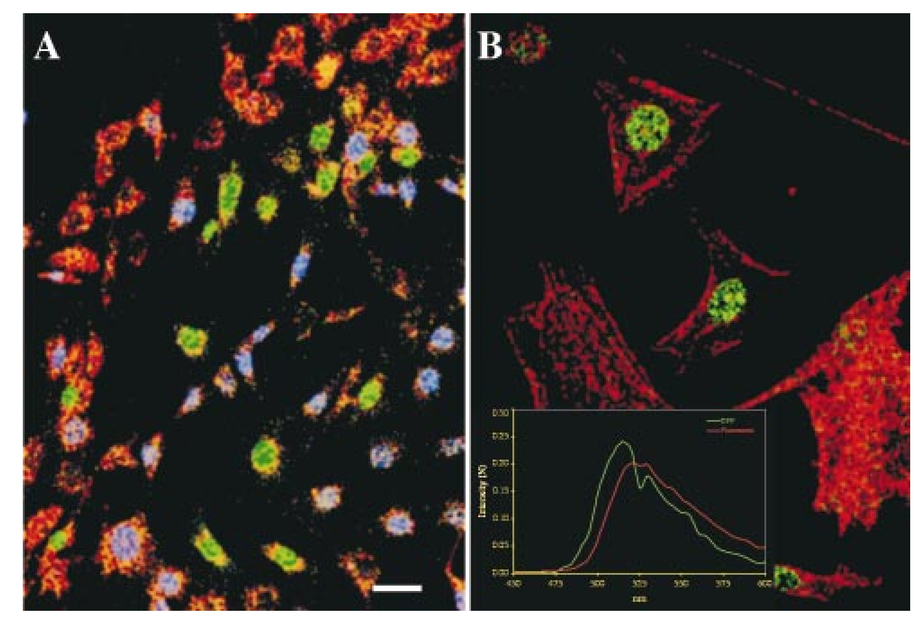

3.4.

Determing the Least Number of Data Points Required to Distinguish Fluorophores

A natural question that follows from these analyses is what instrument bandwidths and how many data points are necessary to separate closely spaced fluorophores such as GFP and YFP. GFP and YFP have similar spectral shapes and are only 15 nm apart in emission maxima [Figure 1(C)]. To this end, we modeled different instrument response functions with the data collected from GFP and YFP expressing cells. To create wider wavelength bins, the spectral data were convolved with LCTF bandwidths from 10 to 30 nm, keeping a sampling grid of 5 nm, and then classified as before. Classification of the spatially segregated data was surprising robust with regard to the filter bandwidths from 10 to 20 nm, but classification began to breakdown for 25–30 nm bandwidths (data not shown). An alternate experimental approach would be to use a LCTF with a different spectral shape that allows a larger bandwidth with reduced spectral crosstalk between data points. For example, a rectangular band pass tunable filter (top hat) would allow more light to pass with less contamination from outside the band pass since it does not sample the spectra in the wings as does the Gaussian line shape of this LCTF. An advantage of a larger bandwidth is that the recorded signal per channel increases (noise decreases) as the sampling window is made larger.

We also analyzed the data to determine the minimum dataset needed to classify the images. We performed a step-wise linear discriminant analysis of the data of Figure 2 to find the minimum number of measurement variables, in our case the number of spectral channels, required to parse the data into a fixed number of disjoint classes. We used the Wilks lambda criterion to select variables to be included or excluded from the analysis, namely the used ratio of the generalized within-class variance to the generalized total variance.¹³ An F test with respect to the ratio of the Wilks statistic for the proposed new set of variables to the Wilks statistic for the current set of variables is used to decide on whether to add a new variable to the set or delete a variable from the set. This test is performed iteratively on the data until there is no observable change in the F statistics.

For the imaging spectrometer data used in our experiments, application of this algorithm resulted in a minimum of 16 noncontiguous spectral channels for robust assignment of image pixels to their correct spectral class. The results show that we can obtain classified images with 16 bands that are equivalent to those resulting for using the full 32-band dataset. For CFP, GFP, and YFP, the optimum bands were 475, 485, and 495–560 nm. Note that this analysis applies only the spatially segregated probes; the minimum dataset for classification may not be the minimum one for spectrally mixed pixels that need to be unmixed. These findings will help us determine the least number of data points requisite to categorize desired fluorophores in order to speed faster data acquisition and lessen storage requirements—both vital considerations for time lapse videomicroscopy.

3.5.

Comparison to Other Approaches

Previous reports of using multiple dichroic filters to separate the excitation and emission wavelengths of different color variants have shown the power of multicolor imaging.^{16 17 18 19} The broadening and blueshifting of the excitation spectra in TPLSM, as well as the difficulties of rapidly shifting the excitation wavelength to optimally excite different forms, complicate the previously published fixed filter approaches.^{16 17 18} Computational approaches to correct spectral bleedthrough work well with relatively well separated labels, but fail to give robust results with many labels. Similarly, such approaches have difficulties in cases in which probe intensities are dramatically mismatched (as in our experiments in which the CFP and YFP signals were weaker than that of GFP as well as the experiments which used exogenous DiI). These techniques also require at least as many filters as probes; therefore, the equipment needed for any system with many probes begins to resemble imaging spectroscopy. Additionally, the spectrally mixed pixels obtained using multiple probes cannot be unmixed by spectrally broad filters; they require the spectral data such as those obtained in these experiments.

The computational approach to spectral overlap with dichroics uses fairly well separated fluorophores and relies on the fact the red, green, and blue filters for a color camera are rather broad. As a result, one can measure how much of DAPI blue, for example, is detected by the red and green color components and construct a deconvolution matrix. We applied this method to our data, using as the data the three slices taken at the emission peaks, 490, 515, and 530 nm, measured the overlap matrix, and applied it to the data. When the individual “corrected” wavelength slices were examined, the comparison with the data classified with the entire image cube was rather poor; i.e., the correction did not isolate each fluorophore into a single band, due to the narrow emission peak spacing. Since so much of the EFP, GFP, and YFP spectra overlap, this approach does not create a usable overlap matrix (for example, half of the CFP signal intensity lies above 515 nm, the peak of the GFP emission).

Recent reports of fluorescent lifetime imaging microscopy (FLIM)¹⁹ offer the potential to separate CFP, GFP, and YFP probes, although still with some spectral cross talk. However, FLIM should show increased error rates in settings where the environment of the dye alters the lifetime, in which dyes are mixed within individual pixels, or in which the intensities of the dye signals are not well matched. While the combination of FLIM with imaging spectroscopy might resolve these challenges, the approaches used here offer robust performance without the challenge of lifetime imaging.

There is one significant limitation to the approach outlined here that should be mentioned. The spectra were obtained band sequentially, requiring multiple scans of each image plane to sample the full spectrum of each pixel. Not only is this data collection slow (it takes 5–14 min to collect a data set), it also increases the exposure of the specimen to the exciting light. Photobleaching is a problem with many of the fluorescent dyes that we tested, but not much of a problem with the GFP color variants. However, the confirmed ability to clearly separate out so many distinct emission spectra validates our experimental approach. Both the rate of data collection and the degree of potential photobleaching will be improved by an instrumental design in which the spectrum is obtained by an array of parallel detectors.

By combining imaging spectroscopy and TPLSM, we were able to concurrently image and distinguish four closely adjoined emission spectrums representing three color variants of GFP and the vital dye DiI. In addition, the demonstrated ability to identify fluorescent species whose spectra differ by only 7 nm (GFP and fluorescein) now allows a larger number of fluorescent probes to be coincidentally followed. The capability to simultaneously image multiple distinctly colored proteins offers obvious advantages, ranging from uniquely following distinct populations of cells by their expression of a particular, to uniquely following an intracellular component tagged with one fluorescent protein even when outnumbered by components tagged with another color. The aforementioned approaches provide a significant step to realizing the dream of dynamically and multispectrally viewing embryogenesis by three-dimensional, time-lapse videomicroscopy, thereby providing an imminent means by which to decipher the multifaceted combinations and interactions that simultaneously occur during the complex signaling cascades and cellular responses that underlie biological processes.