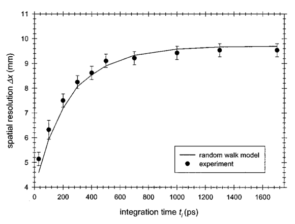
1.

Introduction

Application of nonionizing optical and near-infrared radiation for medical diagnostics attracts widespread interest. It is due to its potential to quantify from noninvasive in vivo spectroscopic measurements local optical characteristics of tissues, thus, discriminating different types of tissues to detect and characterize tumors, cysts, etc. (see the reviews in Refs. 1 and 2). However, strong light scattering in tissue results in inferior spatial resolution for optical techniques relative to those using x ray while imaging abnormalities deeply hidden in the turbid media. Thus, for these techniques, quantification of the size and optical characteristics of the target becomes a critical requirement to be clinically successful. Solution of this problem requires an adequate forward model that can predict measurable parameters (e.g., intensity distributions) for a given distribution of tissue optical characteristics. As for any imaging technique, the point spread function (PSF) is the major component of such a model. It does not only determine achievable spatial resolution, but the knowledge of the PSF is a prerequisite of any reasonable image reconstruction. It is known the inverse algorithms applied to optical imaging are ill posed. Thus, simple analytical expressions for the PSF can save computation time and improve the performance of inverse algorithms, in particular, for time-resolved imaging in which better spatial resolution using photons with shorter time of flight^{3 4 5 6 7} is available. Moreover, by analyzing different time windows of time-of-flight data, one can separate scattering and absorptive perturbations inside a highly scattering medium.⁸

The most detailed theoretical examination of the spatial resolution for time-resolved experiments has been implemented using random walk theory (RWT) in the papers.^{3 6} This analysis involved calculation of the PSF. It was shown that the transillumination PSF of the photons, crossing a homogeneous turbid slab of thickness L and exiting it with different time delays Δt due to scattering as a function of lateral coordinates, is well represented by a Gaussian. Moreover, a simple analytical relationship between a chosen time delay of photons and the width (dispersion) of this Gaussian σ(Δt,z) has been found, where z is the depth of the imaging plane. This width corresponds to the transverse spatial resolution of the system, as a function of depth.

Several sets of experimental data, obtained at University College London, supported the RWT model.⁹ However, up to now two important questions were left concerning experimental verification of the RWT formulas for PSFs. First of all, theoretical dependence of spatial resolution (i.e., the PSF shape) on time delay has been validated experimentally only for the case of midplane imaging (z=L/2), when resolution is expected to be the worst. That was justified, since at the earlier research stages a major interest was in the estimates of the limiting resolution of the time-resolved imaging. However, to solve an inverse problem in the optical imaging, reliable formulas for PSFs at other depths of imaging should be available as well. Second, while simple random walk formulas pertain to the width of the PSF at the given time delay Δt, which is practically important for time-resolved imaging, existing experimental data (e.g. Ref. 9) deal with the integrated signal up to t_i with each time window weighted by a corresponding intensity. That introduces additional errors in the comparison of the theory and experiment. We can directly compare results of these two approaches only for the shortest time delays (on the rapidly growing part of the intensity time-of-flight distribution). Otherwise, preliminary numerical integration of the theoretical formulas is required.

In this paper we use new measurements of spatial resolution at subsequent narrow time windows of δt=50 ps, performed in the University of Naples, to validate random walk formulas for imaging at different depths (z=L/2, L/4, 3L/4). To address the question of possible dependence of time-resolved spatial resolution on the slab thickness, recently discussed in the literature,⁷ we also analyzed experimental data⁷ for a slab that is considerably thinner (L=15 mm) than used in previous experiments (L=50 mm). We have shown that our theoretical expression, not involving such dependence, works well in this case, too.

2.

Experimental Setup

The experimental setup used for the measurements was described in Refs. 10 and 11. An argon laser (Coherent, Model SABRE 40) pumped a mode-locked Ti:Sa laser (Coherent, Model MIRA 900DUAL) with pulse duration of 130 fs, a repetition rate of 76 MHz, and an average power of 1.5 W at 800 nm. A streak camera (Hamamatsu Photonics, Model C5680, S1-IR extended photocathode), working in a synchroscan mode, was used as a detector. To obtain the trigger signal for the streak camera synchroscan sweep, a small fraction of the laser pulse was sent to a photodiode (Hamamatsu, Model C1808). After this the laser light was coupled to two different optical fibers, one for the reference beam and the other for the main beam. Neutral density filters were used to reduce the pulse energy both for triggering, reference and main beams. Collinear geometry of a source-detector pair was realized by alignment of a source fiber with a collecting fiber bundle. The latter had an aperture matching the entrance slit of a streak camera. The scanning of the sample was realized by translating the source-detector axis in 1 mm steps. Curves representing intensity I as a function of time t have been obtained from a two-dimensional charge coupled device response. The full temporal window recorded by the streak camera was about 3 ns. Its temporal resolution depends on the size of an entrance slit and can reach up to a few picoseconds, if the slit is opened at around 20–50 μm. However, to increase a signal/noise ratio for the presented resolution measurements the slit was opened at ∼400 μm providing an overall temporal resolution of the experimental system of ∼30 ps.

To estimate the spatial resolution, we employed a conventional technique based on measurements of the edge-response function (ERF), obtained from a sharp edge of an opaque mask embedded in a scattering slab (see, e.g., Ref. 12). The ERF for a linear system is equal to the integral of the line spread function (LSF). If the LSF of an imaging system can be represented by a Gaussian distribution (as is expected for transillumination through the turbid medium⁶), then the ERF is a Gaussian integral that is well approximated by an inverse polynomial (maximum error is within 0.025). In our case we use a numerical approximation for this Gaussian integral (presented in the software package ISML Fortran 90 MP Library-DIGITAL Visual Fortran-Microsoft) that was found to work better than an inverse polynomial. As a measure of the spatial resolution Δx, we use here full width at half maximum of the LSF, which is equal to 2.35σ. It should be noted that LSF is the spread of a point source due to scattering properties of a medium, when viewed in two dimensions. For an isotropic medium the LSF differs from the PSF only by a constant amplitude factor.³

We have investigated two liquid phantoms made of an aqueous solution of Intralipid that is generally used to simulate the optical properties of biological tissues. The solution was set in an optical glass cuvette (50×143×96.5 mm) that was oriented so that the illuminated surface (one of the two largest sides of the slab) was perpendicular to the beam. The first analyzed sample was a 2 solution of Intralipid 10 (Pharmacia) with distilled water. The absorption and reduced scattering coefficients obtained for this solution by preliminary time-resolved transmittance measurements are μ_s ^′=0.232±0.01 and μ_a=0.0097±0.001 mm ⁻¹. The second sample had considerably higher volume concentration of Intralipid (4 solution of Intralipid 20 with distilled water) to simulate the case of a more turbid medium. Similarly estimated optical coefficients in this case are as follows: μ_s ^′=0.974±0.01 and μ_a=0.0025±0.0001 mm ⁻¹.

The cell dimensions were sufficiently large to avoid appreciable boundary effects, as has been verified experimentally by estimating contribution of photons that reach cuvette side boundary. It proved to be negligible for the considered temporal range. Theoretical analysis, based on the results of a recent paper¹³ confirms this conclusion. In this paper it was shown that for a “zero boundary” condition, the effect of the side boundary at the distance R from the source-detector axis increases with an increasing time delay Δt, and is well approximated by a correction factor K_b=1−exp(−μ_s ^′R²/cΔt), where c is the speed of light in the medium. For a more realistic “extrapolated boundary” condition,¹⁴ the distance R in the above expression for K_b should be replaced by an effective value R _eff =R+d_e, where the shift d_e=1.86/μ_s ^′ for a given mismatch of the index of refraction. Since even for the largest analyzed Δt=1800 ps K_b is very close to unity (∼0.98) for the source-detector axis passing through the cell center, influence of the cell side boundaries can be neglected for our experimental conditions.

The ERF measurements were performed by imaging the edge of a black mask placed at different depths inside the cuvette.

It should be noted that these experiments were not intended to simulate a real situation of diffuse medical imaging. Instead, their aim was to estimate influence of the highly scattering medium on the imaging properties of the time-resolved experimental system. Our findings can be incorporated into the forward model for image reconstruction. Similar approach is common with application of the PSFs for other imaging modalities.

3.

Model Validation

The random walk model (RWM) provides a simple analytical formula for expected spatial resolution of the optical time-resolved imaging system, as a function of mean time delay Δt of photons (assuming a narrow time gate of the detector) and depth z of the target inside the tissue slab of thickness L (Ref. 6)

Figure 1

(a)–(d) The spatial resolution as a function of time delay for different depths of imaging (slab thickness L=50 mm, scattering coefficient μ_s ^′≈0.23 mm ⁻¹).

Due to symmetry our model predicts similar values of spatial resolution for z=0.5L±0.25L. ⁶ As can be seen from Figure 1, experiment supports this assumption.

Comparison between experimental results and predictions of the random walk model for the second analyzed sample (with higher scattering coefficient) (z=0.5 L) also confirms that Eq. (1) provides an adequate estimate of the spatial resolution in the whole analyzed range of time delays (630–2130 ps) (see Figure 2). (Note that the maximum of the corresponding photon pathlength distribution Δt _max ∼1800 ps for this experimental setup is inside this range.)

Figure 2

The spatial resolution as a function of time delay for midplane imaging (slab thickness L=50 mm, scattering coefficient μ_s ^′≈0.97 mm ⁻¹).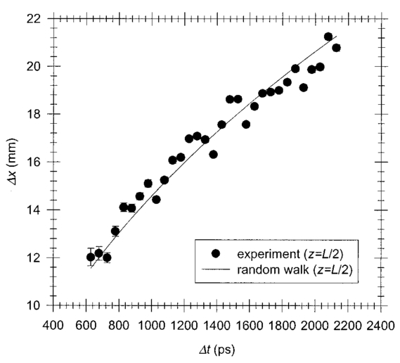

An interesting consequence of the random walk model for time-resolved spatial resolution is that its value for a given time delay and relative depth (z/L) of the target is independent of medium thickness L. This question was discussed in the recent paper.⁷ Authors, analyzing their experimental data on ERF (i.e., integrated signal up to limit time delay t_i ), came to the qualitative conclusion that there is some dependence of resolution on the slab thickness. However, in such a setup to make quantitative comparison of the discussed formula and experimental data is not that straightforward. In fact, at first, the mean time delay of the photons in the broad time window is to be calculated, using corresponding pathlength distribution p(Δt,L), and then it should be substituted instead of Δt into expression (1).³ Since p(Δt,L) strongly depends on L, the mean time delay and measured effective spatial resolution also depend on thickness. All previous quantitative validations of expression (1) were realized with slabs of “standard” thickness L=50 mm. To substantiate our approach for thin slabs, we analyze existing data from Ref. 7, obtained for the thinnest available slab ( L=15 mm, μ_s ^′≈ 0.75 mm ⁻¹ and μ_a≈0.006 mm ⁻¹ ). After simple numerical integration, described in Ref. 3 [Eq. (16)], we found mean time delays for consecutive time windows and corresponding effective spatial resolution (determined in Ref. 7 as corresponding to 10 response on the modulation transfer function) Δx=2.93σ. In Figure 3 our estimates for μ_s ^′=0.7 mm ⁻¹ are presented along with experimental data. Just as in the case of L=50 mm, analyzed before for the same type of solid phantom,^{3 9} agreement proves to be very good over the whole range of time delays (error <15 ).

Figure 3

The spatial resolution at the midplane measured as a function of integration time for a thin slab (L=15 mm).

4.

Summary

Experimental validation of the discussed analytical formula for the time-resolved spatial resolution, as a function of time delay and target depth, is important to estimate the spatial resolution achievable for time-resolved optical imaging. It should be noted that this RWM relation is the only simple theoretical prediction for this significant parameter known in the literature. Previous quite successful tests of the model, such as Ref. 9, were, however, very limited in scope. They were realized only for one type of solid phantoms and tested just the behavior of the midplane resolution, integrated over relatively broad time windows. This time integration is expected to introduce an additional dependence of resolution on the sample thickness L due to significant changes in photon pathlength distributions with variation of L. It proved to be that all data used before for theory validation were obtained for the same value of L=50 mm. To test the relationship between the time-resolved spatial resolution and the slab thickness discussed in Ref. 7, we compared their integration time data for the slab of much smaller thickness ( L=15 mm) with predictions of RWM and found a very good agreement.

In the present paper, for the first time we directly verified Eq. (1) by measurements at subsequent narrow time windows. We also probed the dependence of the resolution on the depth of the imaging plane and found the simple RWM description of this dependence to be quite adequate.

To sum up, we analyzed two independent sets of experimental data for two different phantoms (one of these sets was obtained by the authors and the other was taken from the literature). The results substantiate use of the formula (1) as a simple tool to estimate the expected resolution at different depths and time delays with reasonable accuracy. In combination with the earlier finding of the RWM that the PSF for the time-resolved imaging through a turbid slab is close to a Gaussian, it provides a good starting point for development of the image reconstruction procedures.