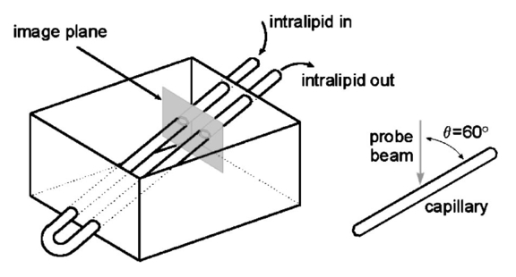
1.IntroductionColor Doppler optical coherence tomography (CDOCT), also called optical Doppler tomography, is a function extension of optical coherence tomography (OCT)1 2 3 that uses motion (flow) in the sample as a contrast mechanism. CDOCT is capable of depth-resolved imaging of flow in turbid media with micron-scale spatial resolution.4 5 6 In vivo imaging of blood flow has previously been demonstrated in animal models.7 8 9 10 11 12 13 14 Recently, in vivo imaging of blood flow in humans has been demonstrated using CDOCT.15 16 17 OCT and CDOCT are based on the technique of low-coherence interferometry, typically using a Michelson interferometer. A broad-bandwidth (low temporal coherence) light source is split by a 50/50 beamsplitter into two paths. The sample to be imaged is placed in one path, while a scanning, retroreflecting optical delay time (ODL) comprises the other path. The light that is backscattered from both paths is recombined at the beamsplitter and collected by a photodetector in the fourth arm of the interferometer. Light from the sample that is pathlength-matched to within the source coherence length was light from the ODL interferes, generating a signal proportional to the localized backscatter in the sample. The light returning from the reference arm is Doppler shifted by the scanning ODL by a frequency fr=2Vr/λ0. Here, Vr is the phase velocity of the ODL scanning and λ0 is the center wavelength of the light source. OCT and CDOCT take advantage of optical heterodyne detection, such that the amplitude of the interferometric signal (interferogram) is proportional to the electric field amplitude of the light returning from the sample, and the carrier frequency corresponds to the reference arm Doppler shift frequency fr. In the same way that reference light is Doppler shifted by the ODL, sample light may be Doppler shifted by moving scatterers in the sample, such as blood cells flowing in vessels. If sample light is backscattered by a moving particle or reflection site, that light is Doppler shifted by a frequency fs=2Vsns cos(θ)/λ0; where Vs is the velocity of the moving scatterer, ns is the local index of refraction in the sample, and θ is the angle of the probe beam with respect to the velocity vector of the moving scatterer. Therefore, the envelope of the interferogram is a profile of the localized reflectivity as a function of depth in the sample, while the localized Doppler shift is encoded in frequency modulation of the carrier. A series of consecutive depth scans can be recorded while the probe beam is translated laterally across the sample resulting in an OCT reflectivity and/or velocity image. CDOCT relies on the identical optical design as OCT, but additional signal processing is used to extract information encoded in the carrier frequency of the interferogram. In the context of imaging biological tissues, CDOCT is motivated by the diagnostic significance of blood flow in many pathological conditions and the potential to monitor therapeutic interventions. CDOCT is currently under investigation for applications in dermatology,14 16 ophthalmology,17 cardiology,8 and gastrointestinal endoscopy.13 For imaging living tissue in situ, a CDOCT system capable of real-time processing will have significant advantages over one that requires processing time, including convenience, mitigation of motion artifact, and the ability to image dynamic flow parameters such as pulsatility. In some clinical situations, such as endoscopy, real-time imaging will be not only advantageous, but necessary. For example, large vessels in and around bleeding peptic ulcers are the targets for therapeutic treatments. These ulcers are only accessible endoscopically, and real-time imaging methods are necessary in order to integrate OCT with endoscopy.19 20 A real-time method to monitor flow during therapy could assist physicians in treating bleeding ulcers while minimizing unnecessary tissue damage and recurrence rates.13 In previous implementations of CDOCT, carrier frequency modulation information has been extracted off line by digital signal processing (DSP) of the acquired image data. The standard DSP method is to perform time-frequency analysis of each A scan using the short-time Fourier transform, although alternative DSP methods have recently been explored.16 18 To date, however, every DSP method has proven to be too computationally intensive to extract velocity information in real time, even when digital data are reduced by using phase sensitive demodulation prior to digitization.9 Although hardware DSP should potentially accelerate the processing, DSP methods have not yet proven to be suitable for real-time CDOCT imaging. The purpose of this work was to implement a CDOCT system capable of performing Doppler flow signal processing in real time in order to integrate the technique with previously described real-time OCT imaging systems.20 21 Our goal was to develop a method of extracting an estimate of the interferogram center frequency by operating directly on the OCT signal as it is required (prior to digitization), allowing direct digitization and display of an image representing localized Doppler shift with little or no postprocessing. This strategy required a fundamentally different signal processing scheme; one which acts directly on the time-domain data without the need for transforms. 2.TheoryAutocorrelation-based signal processing schemes have long been used for real-time flow measurement using ultrasound.22 We have developed a novel autocorrelation-based Doppler processing method for CDOCT23 that is simple in concept and readily realized in analog hardware (Figure 1). In CDOCT, the interferometric signal [the alternating current (ac) component of the photodetector response] can be written as an envelope and carrier where ωg is the carrier angular frequency of the interferogram and t is time. The autocorrelation of the interferogram is a function of delay τ and is defined as the expected value of the product of the interferogram and a delayed version of the interferogramFigure 1Flow diagram of real-time autocorrelation-based CDOCT signal processing. The interferogram (the ac term of the detector response) is bandpass filtered to reduce noise then limited to remove amplitude modulation and retain only phase information. The limited signal is low-pass filtered to remove higher order frequency harmonics then split into two paths. One path is delayed then both are multiplied together then low-pass filtered. The result of these operations, representing the localized flow velocity estimate, is digitized and displayed in real time.  Writing Eq. (2) in terms of the interferogram envelope and carrier and expanding the expression yields Noting that the first term evaluates to zero, and defining the autocorrelation of the envelope as R(τ)=〈g(t)g(t+τ)〉, the autocorrelation of the interferogram can finally be written as Thus, the Doppler shift information encoded in the carrier of the interferogram is present in the carrier of the autocorrelation of the interferogram, which is a function of delay rather than time. We isolate the carrier from the envelope by processing the interferogram with a high-dynamic range limiter before the autocorrelation is measured (Figure 1). This reduces the interferogram envelope to a constant value, and therefore the envelope of the autocorrelation will be constant and only the carrier frequency information will be retained. In order to reduce the autocorrelation to a cosine function of the carrier frequency of the interferogram, a single element of the autocorrelation of the interferogram is computed as lag τ0: From this point forward, we express the autocorrelator response as a function of frequency, as delay is no longer variable. A single lag element of the autocorrelation of the limited interferogram may be readily computed in analog hardware as illustrated in Figure 1. After limiting, the interferogram is split into two paths. One path is delayed by a fixed lag time τ0, and then the signals are multiplied by an analog mixer. A low-pass filter performs the averaging operation of the autocorrelation computation. Optionally, the limited interferogram may be split by a 90° splitter. In this case, the autocorrelation becomes a sine function of the carrier of the interferogram: R˜(ωg)∝sin(ωgτ0). The carrier frequency ωg of the interferogram is the sum of the Doppler shifts from the reference and sample arms We choose fr and τ0 such that cos(2πfrτ0)=0 [or sin(2πfrτ0)=0 in the case of the 90° splitter]. It can then be shown that the autocorrelation reduces to a sinusoidal function of the sample arm Doppler shift fs only In other words, the reference arm Doppler shift and the lag time of the delay line in the single-element autocorrelator are chosen such that the no-flow (fs=0) point of the autocorrelation is located at a zero crossing, as illustrated in Figure 2(a). In this way, a positive value of the autocorrelation represents flow in one direction, and a negative value represents flow in the opposite direction. The shaded regions of Figure 2(a) represent the bandpass filter at the input of the signal-processing network. This filter limits the frequency range that the autocorrelator can measure. If the output of the limiter were conditioned such that the input to the autocorrelator was a square function rather than a sinusoidal function, then the output of the autocorrelator would be a linear function of the Doppler shift rather than a sinusoidal function. The reason for filtering the input to the autocorrelation to a sinusoidal function is because with our current implementation, dispersion in the electronic delay line unacceptably distorts the delayed signal if it contains higher order frequency components. Figures 2(b) and 2(c) illustrate the effect of the length of the lag time τ0 on the output of the autocorrelator. The sensitivity of the autocorrelator to velocity may be defined as the slope of the output of the autocorrelator with respect to fs evaluated at fs=0 (representing no flow): Thus, the velocity sensitivity is proportional to the autocorrelator delay, τ0. The sensitivity may be increased by using a longer delay τ0, but an upper limit is imposed on τ0 by the spatial resolution of the CDOCT system. It is necessary that τ0 not be short enough that the delayed and undelayed signals represent essentially the same position in the tissue. This limit on the velocity sensitivity may be circumvented by correlating adjacent A-scans,6 16 24 effecting a much longer delay, as is commonly done in Doppler ultrasound imaging.22 The monotonic response range of the autocorrelator is the period of the autocorrelator output centered at fs=0: In other words, the range of Doppler shift frequencies resulting in monotonic response is inversely proportional to τ0. The monotonic response range can be written in terms of sample velocity by using the Doppler equation: If the sample flow velocity is high enough to exceed the monotonic response range for a given lag time, then the autocorrelator response will “wrap around” sinusoidally. When the flow velocity range is sufficient to cover several cycles of the autocorrelator response, then “bands” of equal velocity appear in the image, appearing as characteristic colored rings in the color velocity display. The frequency values corresponding to the centers of the rings can also be determined by inspection of Eq. (7). The red and blue bands correspond to sample Doppler shifts of where m is the set of all positive and negative integers. The black bands correspond toUsing the Doppler equation, we determine the velocity values corresponding to the bands. The red and blue bands correspond to sample velocities The black bands correspond to 3.MethodsThe real-time CDOCT system we have developed23 was implemented on a high speed OCT system which has been previously described in detail.21 This system is based on a standard Michelson interferometer configuration (Figure 3). Light from a high-power broadband optical source (10 mW, 47 nm bandwidth centered at 1310 nm) is split by a 50/50 fiber coupler into the reference and sample arms of the interferometer. The reference arm consists of a rapid scanning optical delay (RSOD) line which is based on standard Fourier-domain ultrafast laser pulse shaping techniques. This delay line is capable of a scanning group delay at a very high repetition rate. We have achieved group delay scans corresponding to pathlengths up to 5 mm at depth-scan repetition rates up to 8000 scans per second using resonant scanning mirrors. The RSOD line has the further advantage of providing an additional degree of control over the carrier frequency of the interferogram. The carrier frequency of the interferogram is the reference Doppler shift frequency, which is the rate at which the phase of the reference beam is scanned. In other words, the scan rate of the phase delay (not the group delay) determines the carrier frequency of the interferogram. The group delay gates the image-bearing light returning from the sample, and therefore ranges the scan and determines the bandwidth of the interferogram. For a simple scanning mirror delay line in free space, the phase delay and the group delay are identical. The RSOD line uses first order dispersion to generate a group delay with a dominant term which is independent of phase delay. Phase delay, and therefore the interferogram carrier frequency, may be tuned over a wide range without significantly affecting the group delay (or imaging scan depth). For Doppler measurements, linearity of the scan velocity was essential, so a galvanometric scanning mirror was used with a constant-velocity drive signal and scan repetition rates of 600–800 Hz. Higher scan rates with a constant reference Doppler shift are possible by careful tuning of the galvanometer driver circuitry or by use of a frequency shifter with the RSOD set to zero phase delay scanning and rapid (albeit nonlinear) group delay scanning. A high bandwidth photodetector transduced the optical signal and Doppler signal processing was performed on line in analog hardware in real time. The output of the Doppler signal processing system was digitized by a variable speed frame grabber and color coded and displayed in real time using a desktop computer. The images were simultaneously recorded to high quality (S–VHS) video tape. It should be noted that CDOCT data are recorded simultaneously with OCT data such that both data sets are available for concurrent display and recording. In the future we will implement real-time composite color Doppler OCT by color coding and overlaying CDOCT data on corresponding OCT images. Figure 3Block diagram of real-time CDOCT system. A 10 mW broadband (47 nm) optical source centered at 1310 nm illuminates the fiber-optic Michelson interferometer. A Fourier-domain rapid scanning optical delay line comprises the reference arm. The sample is scanned laterally with a galvanometric X–Y scan head. Signal processing to extract the Doppler shift information is performed on line in analog hardware. The signal is digitized by a variable scan frame grabber and displayed and recorded to high quality video tape in real time.  In practice, it is difficult to precisely tune the autocorrelator delay line to match the no-flow/zero-crossing condition. It is more practical to choose a delay line of approximately the desired lag time, then tune the reference arm Doppler shift frequency to match the zero-crossing condition. The reference arm Doppler shift frequency may be tuned by varying the scan rate of the phase delay of the reference light by the optical delay line in the reference arm of the interferometer. In this application, it is an extremely useful feature of the Fourier-domain RSOD line that the scan rate of the phase delay may be tuned without significantly affecting the scan rate of the group delay.21 In other words, fr may be broadly tuned without significantly affecting the imaging depth scan range at a given scan repetition rate. For testing the system, a simple tissue-simulating phantom was constructed consisting of 2 intralipid solution flowing in glass capillary tubes, as illustrated in Figure 4.23 The tubes were parallel and connected with a sealed tube such that the flow in each was of equal magnitude and opposite direction. The imaging beam made an angle of 60° with the capillaries. Flow velocity was continuously controllable with a valve. For demonstrating real-time imaging of blood flow, an animal model was prepared according to a protocol approved by the Institutional Animal Care and Use Committee of the University of Hospitals of Cleveland. A rat was anesthetized with a 3:4 ratio of ketamine and xylazine, 0.1 mL/100 g. An approximately 1 cm square section of skin from the hindlimb was removed, revealing the femoral artery. Throughout imaging, the surgical site was irrigated with isotonic saline to prevent drying of the exposed tissue. The incidence angle of the OCT beam on the tissue was approximately 30° but was not held fixed due to respiration of the animal. Therefore, the blood flow velocity was imaged, but not quantified absolutely. 4.ResultsFigure 5 displays a series of still frames extracted from recordings of the bidirectional flow phantom with the real-time CDOCT system. The signal proportional to the instantaneous carrier frequency is displayed in a false color scale common for flow imaging, so that black represents no flow, red represents flow in one direction, and blue represents flow in the opposite direction. A smooth flow velocity profile, consistent with laminar flow, is evident in the images of the phantom, as expected. The image size is 2 mm vertically (depth) and 4 mm horizontally. The images were recorded at four frames per second with 150 lines per frame and 300 pixels per line. As described earlier, when flow in the sample induces a Doppler shift that exceeds the monotonic response range of the autocorrelator, the signal “wraps around” to display the ringed features shown in Figure 5(d). The flow velocities represented by these equivelocity bands are exactly known, and are determined by fr and τ0. The data shown in Figures 5 and 6 were recorded with fr=375 kHz and τ0=2 μs. Thus, in this case, the monotonic response range [from Eq. (9)] is −125 kHz⩽fs⩽125 kHz. In the phantom, this corresponds to −123 mm/s⩽Vs⩽123 mm/s [Eq. (10)]. Equations (11 12) can be used to calculate the Doppler shifts represented by the red, blue, and black bands. Equations (13 14) can be used to calculate the corresponding velocity values. In the capillary imaged on the right in Figure 5(d), for example, the bands are assigned as follows, starting from the outside: red=125 kHz (123 mm/s), black=250 kHz (246 mm/s), blue=375 kHz (369 mm/s), black=500 kHz (492 mm/s), red=625 kHz (616 mm/s), black=750 kHz (739 mm/s), and blue=875 kHz (8862 mm/s). The capillary imaged on the left in Figure 5(d) contains flow equal in velocity with the capillary on the right but in the opposite direction, so the bands represent values of equal magnitude but opposite sign. Note that the second colored band (red=−375 kHz) is missing. This is because the reference Doppler shift was 375 kHz, so the interferogram here was centered at dc and was filtered out by the bandpass filter after the detector. These bands may prove to be a desirable display method in some applications, especially where it is useful to quantify flow immediately by inspection of the display. The artifacts appearing above and below the tubes, especially on the right, are believed to be due to black level clamping by the image acquisition hardware. The minimum detectable sample Doppler shift fs min is inversely proportional to τ0 and to the SNR of the autocorrelation network. In the configuration described above, fs min was experimentally determined to be approximately 21 kHz (corresponding to 20 mm/s flow velocity in the phantom). This correlates reasonably well with the expected fs min of 16 kHz based on the measured SNR of 5 for the autocorrelator. The minimum detectable sample Doppler shift was limited by the SNR of the autocorrelator, which was primarily limited by loss and dispersion in the autocorrelator delay line. Figure 5OCT and color Doppler OCT images of laminar flow in phantom captured from real-time recording (four frames per second). An OCT image of the phantom (intralipid in glass capillaries) is shown in (a), a CDOCT image with no flow is shown in (b), flow of approximately 130 mm/s in (c), and flow of approximately 860 mm/s in (d), In (b)–(d), the signal proportional to instantaneous carrier frequency is represented in a false color scale, such that black represents no flow, red represents flow in one direction, and blue represents flow in the other direction. The image size is 2 mm vertically (depth) and 4 mm horizontally. As noted, flow that exceeds the monotonic response range for a given autocorrelator configuration can cause the signal to wrap around resulting in the ringed equivelocity features imaged in (d). The artifacts appearing above and below the tubes, especially on the right, are believed to be due to black level clamping by the image acquisition hardware. A slight gradient is apparent in (b) that is due to nonlinearity in the reference delay scan rate. 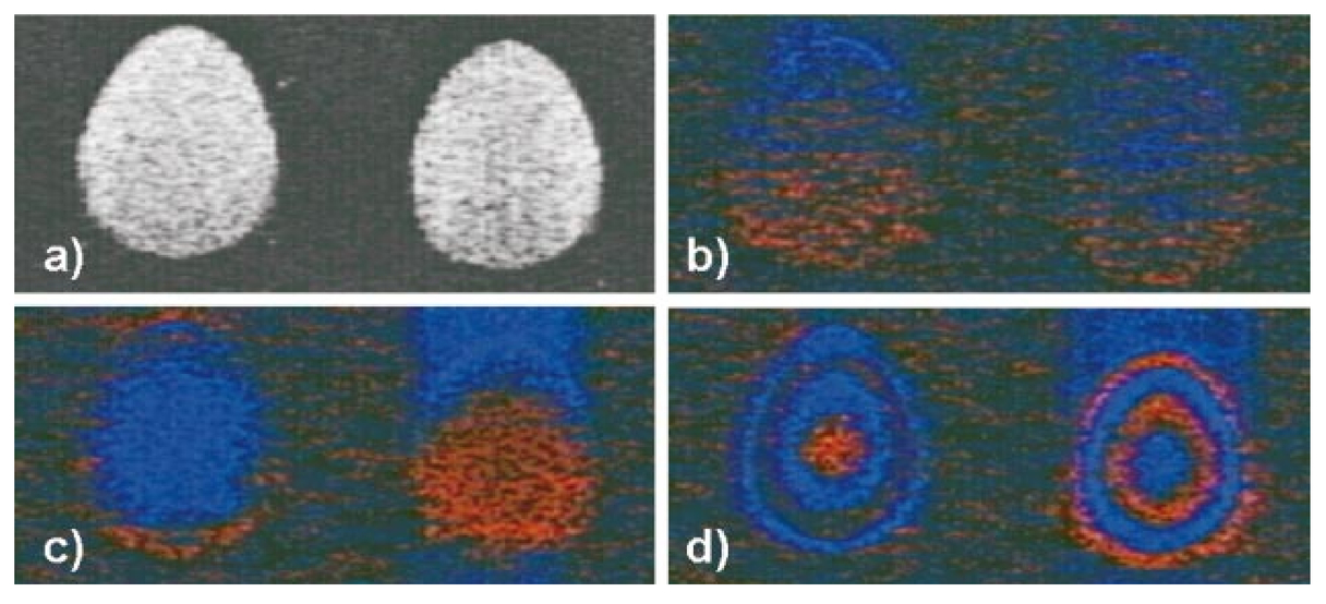 Figure 6Single frames captured from real-time CDOCT recording of blood flow in a rat femoral artery. The image size is approximately 1 mm vertically (depth) and 2 mm horizontally. An OCT image (reflectivity shown in grayscale) of the sample is shown in (a), where the artery can be seen embedded in connective tissue. The flow profile in the artery at three different stages of the cardiac cycle are shown in (b), (c), and (d). Also shown in (b), (c), and (d) are 1D velocity profiles (arbitrary units) extracted horizontally from the center of each 2D velocity profile. Each frame was recorded in 125 ms (eight frames per second). The OCT image (a) is the average of four consecutive images. 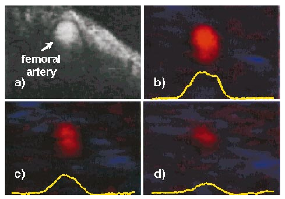 After testing the system using the bidirectional flow phantom, real-time CDOCT imaging of blood flow in vivo was demonstrated in the rat model. Our real-time CDOCT imaging system was used to simultaneously record structure and flow images at eight frames per second (125 ms per image) with 100 depth scans per image. Figure 6 shows single frames captured from the video recording of this experiment. The image size is approximately 1 mm vertically (depth) and 2 mm horizontally. An OCT image of the sample is shown in Figure 6(a), where the artery can be seen embedded in connective tissue. The OCT image is the average of four consecutive images (the system computed a four-frame running average updated at eight frames per second). The Doppler OCT images are not frame averaged. Unfortunately, the real-time visualization of the pulsatile blood flow cannot be appreciated in still images, but the flow profile in the artery at three different stages of the cardiac cycle are shown in Figures 6(b), 6(c), and 6(d). Also shown in Figures 6(b), 6(c), and 6(d) are one-dimensional (1D) velocity profiles (arbitrary units) extracted horizontally from the center of each two-dimensional (2D) velocity profile. By comparing Figure 6(a) with Figure 6(b), it can be seen that the velocity image actually gives a truer image of the artery dimensions than the OCT image. This is because blood strongly attenuates the probe light such that the bottom border of the artery is not clear in the OCT image. The blood flow velocity was not absolutely quantified by careful calibration with independent flow measurement for validation, nor was the incidence angle of the probe beam on the artery carefully fixed because of the respiration and motion of the living animal. Nevertheless, as described earlier, the velocity values can be approximately determined from the system parameters. We roughly estimate that the peak velocity at systole measured in this experiment was about 150 mm/s. Although published measurements of flow rates in a rat femoral artery vary widely, this rate falls within the range of reported values (see for example Refs. 25 and 26). This is the first demonstration to our knowledge of real-time imaging of a two-dimensional blood flow profile in a living sample using CDOCT or any other optical modality. 5.ConclusionsWe have demonstrated imaging of bidirectional flow with CDOCT in real time in a tissue-simulating phantom consisting of intralipid solution flowing in glass capillaries. We have also demonstrated real-time imaging of pulsatile blood flow in vivo in an animal model. A novel autocorrelation technique for the real-time calculation of velocity data was introduced, and its properties in terms of velocity sensitivity and velocity range were discussed, as well as potential applications of real-time CDOCT. Preliminary experiments indicate that the system is flexible and easily configurable, and preliminary results are encouraging that the system may be applicable to clinical in vivo flow imaging. AcknowledgmentsThis research was supported in part by Grant Nos. BES-9624617 and BES-9872829 from the National Science Foundation, and Grant No. R24 EY13015-01 from the National Institutes of Health. A. Rollins acknowledges support from an Olympus Graduate Fellowship. S. Yazdanfar acknowledges support from a NIH Training Grant. Brian Wolf and Volker Westphal are acknowledged for their valuable technical contributions. REFERENCES
D. Huang
,
E. A. Swanson
,
C. P. Lin
,
J. S. Schuman
,
W. G. Stinson
,
W. Chang
,
M. R. Hee
,
T. Flotte
,
K. Gregory
,
C. A. Puliafito
, and
J. G. Fujimoto
,
“Optical coherence tomography,”
Science , 254
(5035), 1178
–1181
(1991). Google Scholar
J. A. Izatt
,
M. D. Kulkarni
,
H.-W. Wang
,
K. Kobayashi
, and
M. V. Sivak
,
“Optical coherence tomography and microscopy in gastrointestinal tissues,”
IEEE J. Sel. Top. Quantum Electron. , 2
(4), 1017
–1028
(1996). Google Scholar
J. M. Schmitt
,
“Optical coherence tomography (OCT): A review,”
IEEE J. Sel. Top. Quantum Electron. , 5
(4), 1205
–1215
(1999). Google Scholar
Z. Chen
,
T. E. Milner
,
D. Dave
, and
J. S. Nelson
,
“Optical Doppler tomographic imaging of fluid flow velocity in highly scattering media,”
Opt. Lett. , 22
(1), 64
–66
(1997). Google Scholar
J. A. Izatt
,
M. D. Kulkarni
,
K. Kobayashi
,
M. V. Sivak
,
J. K. Barton
, and
A. J. Welch
,
“Optical coherence tomography for biodiagnostics,”
Opt. Photonics News , 8 41
–47
(1997). Google Scholar
Z. Chen
,
T. E. Milner
,
S. Srinivas
,
X. Wang
,
A. Malekafzali
,
M. J. C. van Gemert
, and
J. S. Nelson
,
“Noninvasive imaging of in vivo blood flow velocity using optical Doppler tomography,”
Opt. Lett. , 22 1119
–1121
(1997). Google Scholar
J. A. Izatt
,
M. D. Kulkarni
,
S. Yazdanfar
,
J. K. Barton
, and
A. J. Welch
,
“In vivo bidirectional color Doppler flow imaging of picoliter blood volumes using optical coherence tomography,”
Opt. Lett. , 22
(18), 1439
–1441
(1997). Google Scholar
S. Yazdanfar
,
M. D. Kulkarni
, and
J. A. Izatt
,
“High resolution imaging of in vivo cardiac dynamics using color Doppler optical coherence tomography,”
Opt. Express , 1
(13), 424
–431
(1997). Google Scholar
Z. Chen
,
T. E. Milner
,
X. Wang
,
S. Srinivas
, and
J. S. Nelson
,
“Optical Doppler tomography: Imaging in vivo blood flow dynamics following pharmacological intervention and photodynamic therapy,”
Photochem. Photobiol. , 67
(1), 56
–60
(1998). Google Scholar
J. K. Barton
,
A. J. Welch
, and
J. A. Izatt
,
“Investigating pulsed dye laser-blood vessel interaction with color Doppler optical coherence tomography,”
Opt. Express , 3
(6), 251
–256
(1998). Google Scholar
S. Yazdanfar
,
M. D. Kulkarni
,
R. C. K. Wong
,
M. V. Sivak
,
J. Willis
,
J. K. Barton
,
A. J. Welch
, and
J. A. Izatt
,
“Diagnostic blood flow monitoring during therapeutic interventions using color Doppler optical coherence tomography,”
Proc. SPIE , 3251 126
–132
(1998). Google Scholar
J. K. Barton
,
J. A. Izatt
,
M. D. Kulkarni
,
S. Yazdanfar
, and
A. J. Welch
,
“Three-dimensional reconstruction of blood vessels from in vivo color Doppler optical coherence tomography images,”
Dermatology , 198
(4), 355
–361
(1999). Google Scholar
S. Yazdanfar
,
A. M. Rollins
, and
J. A. Izatt
,
“In vivo imaging of blood flow in human retinal vessels using color Doppler optical coherence tomography,”
Proc. SPIE , 3598 177
–184
(1999). Google Scholar
Y. Zhao
,
Z. Chen
,
C. Saxer
,
J. F. deBoer
, and
J. S. Nelson
,
“Phase-resolved optical coherence tomography and optical Doppler tomography for imaging blood flow in human skin with fast scanning speed and high velocity resolution,”
Opt. Lett. , 25
(2), 114
–116
(2000). Google Scholar
S. Yazdanfar
,
A. M. Rollins
, and
J. A. Izatt
,
“Imaging and velocimetry of the human retinal circulation with color Doppler optical coherence tomography,”
Opt. Lett. , 25
(19), 1448
–1450
(2000). Google Scholar
T. G. van Leeuwen
,
M. D. Kulkarni
,
S. Yazdanfar
,
A. M. Rollins
, and
J. A. Izatt
,
“High-flow-velocity and shear-rate imaging by use of color Doppler optical coherence tomography,”
Opt. Lett. , 24
(22), 1584
–1586
(1999). Google Scholar
B. E. Bouma
and
G. J. Tearney
,
“Power-efficient nonreciprocal interferometer and linear-scanning fiber-optic catheter for optical coherence tomography,”
Opt. Lett. , 24
(8), 531
–533
(1999). Google Scholar
A. M. Rollins
,
R. Ung-Arunyawee
,
A. Chak
,
R. C. K. Wong
,
K. Kobayashi
,
J. M. V. Sivak
, and
J. A. Izatt
,
“Real-time in vivo imaging of human gastrointestinal ultrastructure using endoscopic optical coherence tomography with a novel efficient interferometer design,”
Opt. Lett. , 24 1358
–1360
(1999). Google Scholar
A. M. Rollins
,
M. D. Kulkarni
,
S. Yazdanfar
,
R. Un-arunyawee
, and
J. A. Izatt
,
“In vivo video rate optical coherence tomography,”
Opt. Express , 3
(6), 319
–229
(1998). Google Scholar
C. Kasai
,
K. Namekawa
,
A. Koyano
, and
R. Omoto
,
“Real-time two-dimensional blood flow imaging using an autocorrelation technique,”
IEEE Trans. Sonics Ultrason. , SU-32
(3), 458
–463
(1985). Google Scholar
A. M. Rollins
,
S. Yazdanfar
,
R. Un-arunyawee
, and
J. A. Izatt
,
“Real-time color Doppler optical coherence tomography using an autocorrelation technique,”
Proc. SPIE , 3598 168
–176
(1999). Google Scholar
S. Yazdanfar
,
A. M. Rollins
, and
J. A. Izatt
,
“Ultrahigh velocity resolution imaging of the microcirculation in vivo using color Doppler optical coherence tomography,”
Proc. SPIE , 4251 156
–164
(2001). Google Scholar
W. F. Blair
,
L. Chang
,
D. R. Pedersen
,
R. H. Gabel
, and
L. D. Bell
,
“Hemodynamics after autogenous, interpositional grafting in small arteries,”
Microsurgery , 7
(2), 84
–86
(1986). Google Scholar
T. Mohr
,
T. K. Akers
, and
H. C. Wessman
,
“Effect of high voltage stimulation on blood flow in the rat hind limb,”
Phys. Ther. , 67
(4), 526
–533
(1987). Google Scholar
|


CITATIONS
Cited by 82 scholarly publications and 41 patents.
Doppler effect
Optical coherence tomography
Imaging systems
Real time imaging
Digital signal processing
In vivo imaging
Blood circulation


