Review of polarization sensitive optical coherence tomography and Stokes vector determination

Johannes F. de Boer; Thomas E. Milner

doi:10.1117/1.1483879

1 July 2002 Review of polarization sensitive optical coherence tomography and Stokes vector determination

Johannes F. de Boer, Thomas E. Milner

Author Affiliations +

Journal of Biomedical Optics, Vol. 7, Issue 3, (July 2002). https://doi.org/10.1117/1.1483879

1. Introduction

1.1.

Optical Coherence Tomography and Polarization-Sensitive Optical Coherence Tomography

Optical coherence tomography (OCT) is a new technique for high resolution imaging of tissue reflectivity in two or three dimensions to a depth of 2 mm.¹ OCT instrumentation uses a spectrally broadband light source and a two-beam interferometer (e.g., Michelson) with the reflector in one path (i.e., sample arm) replaced by a turbid medium. Depth ranging in the turbid medium is possible because interference fringes are observed only for light in sample and reference arms that has traveled equal optical path lengths to within the source coherence length (2–15 μm). By scanning optical path length in the reference arm and amplitude detection of the interference fringes, a depth scan (A scan) can be recorded that maps sample reflectivity. Temporal coherence length of the source light determines axial resolution of a system, while numerical aperture of the focusing optics determines lateral resolution. Lateral scanning mechanisms allow two- and three-dimensional recording of images from consecutive A scans. Although light is frequently treated as a scalar wave many applications require a description using transverse electromagnetic waves. The transverse nature of light is distinguished from longitudinal waves (e.g., sound), by the extra degree of freedom, which is indicated by the polarization state of light. Polarization sensitive OCT (PS–OCT) uses the information encoded in the polarization state of the recorded interference fringe intensity to provide additional contrast in images of the sample under study. PS–OCT provides high resolution spatial information on the polarization state of light reflected from tissue that is not discernible using existing diagnostic optical methods. In this review paper the authors describe theory and calculation of the Stokes vectors in more detail than that provided in our early reports.² ³ Application of PS–OCT to contemporary biomedical imaging problems is discussed.

1.2.

Optical Properties of Tissue That Influence Polarization

Scattering is the principle mechanism that modifies the polarization state of light propagating through biological tissue. The polarization state of light after a single scattering event depends on the scatterer, direction of scatter and incident polarization state (e.g., Refs. 4 5 6 7). In many turbid media such as tissue, scattering structures have a large variance in size and are distributed/oriented in a complex and sometimes apparently random manner. Because each scattering event can modify the incident polarization state differently, the scrambling effect of single scattering events accumulates, until finally the polarization state is completely random (i.e., uncorrelated with the incident polarization state). A detailed description of the scrambling effect of polarized light in heterogeneous media is given by Brosseau.⁸

An important exception is when the media consists of organized linear structures, such as fibrous tissues that can exhibit form birefringence. Many biological tissues exhibit form birefringence, such as tendons, muscle, nerve, bone, cartilage, and teeth. Form birefringence arises when the relative optical phase between orthogonal polarization components is nonzero for forward scattered light. After multiple forward scattering events, relative phase difference accumulates and a delay (δ) similar to that observed in birefringent crystalline materials (e.g., calcite) is introduced between orthogonal polarization components. For organized linear structures, the increase in phase delay may be characterized by a difference (Δn) in the effective refractive index for light polarized along, and perpendicular to, the long axis of the linear structures. The phase retardation, δ, between orthogonal polarization components is proportional to the distance (x) traveled through the birefringent medium

Eq. (1)

δ = \frac{2 π Δ nx}{λ} .

The advantage in using PS–OCT is the enhanced contrast and specificity in identifying structures in OCT images by detecting induced changes in the polarization state of light reflected from the sample. Moreover, changes in birefringence may, for instance, indicate changes in functionality, structure, or viability of tissues.

2. Theory

2.1.

Historical Context

Use of broadband light in polarization sensitive interferometry has a long history dating back to the founding experimental work establishing our modern understanding of light. For example, use of broadband light in interferometry can be traced to the 16th century when Sir Isaac Newton observed interference rings when two glass plates with different radii of curvature are placed in mechanical contact. Fresnel and Arago performed double slit interference experiments in 1817 that subsequently were interpreted correctly by Thomas Young. Results of the experiment were codified into the Fresnel–Arago laws for interference of polarized light and indicated that light consists of two orthogonal transverse oscillations.⁹ Thirty-five years later Sir George Stokes formulated his description of polarized light [Eq. (20) and sequence] by analyzing similar double slit interference experiments performed by Sir John Herschel. A convenient experimental setup to demonstrate the Fresnel–Arago laws was described by Henry.¹⁰

Application of laser interferometry to characterize the polarization state of light reflected from optical components was reported by Hazebroek and Holscher in 1973.¹¹ More recently, bright broadband light sources that emit in a single spatial mode have provided the basis for novel applications in testing of optical components and biomedical imaging. For example, Newson et al.;¹² constructed a combined Mach–Zehnder/Michelson interferometer (configured in tandem) that used a low coherence semiconductor light source and polarization sensitive detection to measure temperature changes in a birefringent fiber. Kobayashi et al.;¹³ reported an early demonstration of a polarization-sensitive fiber Michelson interferometer using a low coherence light source for testing optical components.

Much emphasis in OCT has been on the reconstruction of two-dimensional maps of tissue reflectivity while neglecting the polarization state of light. In 1992, Hee et al.;¹⁴ reported an OCT system able to measure the changes in the polarization state of light reflected from a sample. Using an incoherent detection technique, they demonstrated birefringence sensitive ranging in a wave plate, an electro-optic modulator, and calf coronary artery. In 1997, the first two-dimensional images of birefringence in bovine tendon were presented, and the effect of laser induced thermal damage on tissue birefringence was demonstrated,² followed in 1998 by a demonstration of the birefringence in porcine myocardium.¹⁵ To date, polarization sensitive OCT measurements have attracted active interest from several research groups.

2.2.

Experimental Configuration

The theory of PS–OCT will be discussed in the context of a Michelson interferometer presented by Hee et al.;¹⁴ Our analysis is a simplified version of the derivation that lead to Eq. (2) in Ref 2. Figure 1 shows a schematic of this PS–OCT system that was used to record all images presented in this paper. A general discussion of polarization effects in two-beam interferometers is given by Steel¹⁶ and analyzed by Bernabeu and Sanchez-Soto.¹⁷ Light with a short coherence length passes through a polarizer (P) to select a pure linear horizontal input state, and is split into reference and sample arms by a polarization insensitive beamsplitter (BS). Light in the reference arm passes through a zero order quarter wave plate (QWP) oriented at a 22.5° angle to the incident horizontal polarization. Following reflection from a mirror or retroreflector, and return pass through the QWP, light in the reference arm has a linear polarization at a 45° angle with respect to the horizontal. Light in the sample arm passes through a QWP oriented at a 45° angle to the incident horizontal polarization and through focusing optics, producing circularly polarized light incident on the sample. Reflected light from the sample, in an arbitrary (elliptical) polarization state determined by the optical properties of the sample, returns through the focusing optics and the QWP. After recombination in the detection arm, the light is split into its horizontal and vertical components by a polarizing beamsplitter (PBS) and focused on pinholes or single mode fibers to detect a single polarization state and spatial mode.

Figure 1

Schematic of the PS–OCT system. SLD: superluminescent diode, 0.8 mW output power, central wavelength λ=856 nm and spectral FWHM Δλ=25 nm, L: lens, P: polarizer, BS: beam splitter, QWP: quarter wave plate, NDF: neutral density filter, PBS: polarizing beam splitter, and PZT: piezoelectric transducer. Two-dimensional images were formed by either axial movement of the sample with constant velocity v=1 mm/s ( z direction), repeated after each 10 μm lateral displacement ( x direction), or lateral movement of the sample with constant velocity v=1 mm/s ( x direction), repeated after each 10 μm axial displacement ( z direction). The latter allows for focus tracking in the sample.

Two-dimensional images can be formed by lateral or axial movement of the sample at constant velocity v, repeated after each axial or lateral displacement, respectively. The carrier or interference fringe frequency can be generated by axial movement of the sample or reference mirror, by translating the reference mirror mounted on the piezoelectric transducer over a few wavelengths, or by a combination of both. Transverse and axial image resolutions are determined by, respectively, the beam waist at the focal point and the coherence length of the source.

2.3.

Jones Matrix Formalism

The polarization state in each arm of the interferometer is computed using the Jones matrix formalism, which has an implicit spectral dependence.¹⁸ The intensity detected in each polarization channel can be described by a two-dimensional intensity vector I, where the two components describe the horizontal (x) and vertical (y) polarized intensities, respectively. The intensities at the detectors are given by

Eq. (2)

〈 I (Δ z) 〉 = 〈 I_{r} 〉 + 〈 I_{s} 〉 + 〈 \begin{matrix} E_{r x}^{*} E_{s x} (Δ z) \\ E_{r y}^{*} E_{s y} (Δ z) \end{matrix} 〉 + 〈 \begin{matrix} E_{r x} E_{s x}^{*} (Δ z) \\ E_{r y} E_{s y}^{*} (Δ z) \end{matrix} 〉,

where E and E^* are the electric field component and its complex conjugate, Δz is the path length difference between reference (r) and sample (s) arms of the interferometer. The angular brackets denote time averaging. The last two terms of Eq. (2) correspond to the interference between reference and sample arm light. After the polarizer, horizontally polarized source light is described by the Jones vector

Eq. (3)

E (z) = E (z) (\begin{matrix} 1 \\ 0 \end{matrix}) .

In our analysis, the electric field amplitude is represented by a complex analytic function,¹⁹ E(z), with

Eq. (4)

E (z) = \int \tilde{e} (k) exp (- ikz) dk,

e˜(k) is the field amplitude as a function of free space wave number k=2π/λ, with

Eq. (5)

\tilde{e} (k) = 0 if k < 0 .

From the Wiener–Khintchine theorem, it follows:

Eq. (6)

〈 {\tilde{e}}^{*} (k) \tilde{e} (k^{'}) 〉 = S (k) δ (k - k^{'}),

which defines e˜(k) in terms of the source power spectral density S(k). The beamsplitter divides the incident light by amplitude evenly between both arms of the interferometer, and the Jones vector describing the light that enters the sample and reference arm is given by

Eq. (7)

E_{si} (z) = E_{ri} (z) = \frac{E (z)}{\sqrt{2}} (\begin{matrix} 1 \\ 0 \end{matrix}) .

First, the polarization state of light reflected from the reference arm is calculated. The Jones matrix for a QWP with fast and slow axes aligned along horizontal and vertical axes is given by

Eq. (8)

QWP = (\begin{matrix} e^{i π / 4} & 0 \\ 0 & e^{- i π / 4} \end{matrix}) .

A QWP with its fast optic axis at an angle ϕ with the horizontal is found by applying a rotation to the Jones matrix in Eq. (8), QWP(ϕ)=R(ϕ)QWP R(−ϕ), with R(ϕ) given by

Eq. (9)

R (ϕ) = (\begin{matrix} cos (ϕ) & - sin (ϕ) \\ sin (ϕ) & cos (ϕ) \end{matrix}) .

The polarization state of light reflected from the reference into the detection arm is given by

Eq. (10)

E_{r} (z_{r}) = R (22.5) \cdot {(QWP)}^{2} \cdot R (- 22.5) E_{ri} = \frac{1}{2} E (2 z_{r}) (\begin{matrix} 1 \\ 1 \end{matrix}),

which describes a linear polarization state at an angle of 45° with the horizontal. The horizontal and vertical components of the electric field have equal amplitude and phase. To calculate the polarization state of light reflected from the sample arm, we assume that the optical properties of the sample can be described by a homogeneous linear retarder with a constant orientation of the optic axis. The Jones matrix of the sample, B(z,Δn,α), is written as a product of average phase delay in the sample, rotation matrices, and the Jones matrix of a linear retarder with the fast axis along the horizontal

Eq. (11)

B (z, Δ n, α) = e^{- ikz \bar{n}} R (α) (\begin{matrix} e^{ikz Δ n / 2} & 0 \\ 0 & e^{- ikz Δ n / 2} \end{matrix}) R (- α),

with kzn¯ the average phase delay of a wave propagating to depth z and n¯ the average refractive index along the fast (n_f) and slow (n_s) optic axes, n¯=(n_f+n_s)/2. Δn=n_s−n_f is the difference in refractive index along the fast and slow axes, and α is the angle of the fast axis with the horizontal. The single pass retardation δ for the Jones matrix B(z,Δn,α) is δ=kzΔn. The Jones vector of the light reflected from the sample arm is given by the product of the optical elements in the sample arm and the incident field vector

Eq. (12)

\begin{matrix} E_{s} (z_{s} + z) & = & Q W P (45) \cdot B (z, Δ n, α) \sqrt{R (z)} B (z, Δ n, α) Q W P (- 45) E_{s i} \\ \propto & \sqrt{R (z)} \int \tilde{e} (k) exp [- 2 i k (z_{s} + z \bar{n})] \times [\begin{matrix} e^{2 i α} sin (k z Δ n) \\ cos (k z Δ n) \end{matrix}] d k, \end{matrix}

with R(z) a scalar that describes the reflectivity at depth z and the attenuation of the coherent beam by scattering, and z_s is the optical path length of the arm up to the sample surface. Using the Wiener–Khintchine theorem [Eq. (6)], the interference terms in the horizontally and vertically polarized channels are given by, respectively,

Eq. (13)

\begin{array}{l} A_{H} (z, Δ z) & = & E_{r x}^{*} E_{s x} + E_{r x} E_{s x}^{*} \\ \propto & \sqrt{R (z)} \int sin (k z Δ n) cos (2 k Δ z + 2 α) S (k) d k, \\ A_{V} (z, Δ z) & = & E_{r y}^{*} E_{s y} + E_{r y} E_{s y}^{*} \\ \propto & \sqrt{R (z)} \int cos (k z Δ n) cos (2 k Δ z) S (k) d k, \end{array}

with z the depth in the tissue and Δz the optical path length difference between sample and reference arms, Δz=z_r−z_s−zn¯. A Gaussian power spectral density is assumed for the source

Eq. (14)

S (k) \propto exp [- {(\frac{k - k_{0}}{κ})}^{2}],

with the full width at half maximum (FWHM) spectral bandwidth of the source given by

κ 2 \sqrt{\ln 2.}

The integration over k in Eq. (13) can be performed analytically, and in the approximation that κzΔn≪1, the expressions simplify to

Eq. (15)

A_{H} (z, Δ z) \propto \sqrt{R (z)} sin (k_{0} z Δ n) cos (2 k_{0} Δ z + 2 α) \times exp [- {(Δ z / Δ l)}^{2}],

A_{V} (z, Δ z) \propto \sqrt{R (z)} cos (k_{0} z Δ n) cos (2 k_{0} Δ z) \times exp [- {(Δ z / Δ l)}^{2}],

with the FWHM of the interference fringes envelope given by

Δ l 2 \sqrt{\ln 2} :

Eq. (16)

Δ l = \frac{1}{κ} = \frac{λ_{0}^{2} \sqrt{ln 2}}{π Δ λ},

and Δλ the spectral FWHM of the source in wavelength. The terms in Eq. (15) for the interference fringe intensities in the horizontal and vertical channels describe the reflected amplitude at depth z, the slow oscillation due to the birefringence k₀zΔn, the Doppler shift or carrier frequency generated by the variation of the optical path length difference between sample and reference arms, and the interference fringes envelope, respectively. The spatial resolution is determined by the width Δl of the interference fringe envelope. Using Eq. (16), the condition κzΔn≪1 is reformulated as zΔn≪Δl, which can be interpreted as a condition that the optical path length difference between light polarized along the fast and slow optic axes of the sample should be smaller than the coherence length of the source.² Schoenenberger et al.; have given a similar derivation, assuming the phase retardation δ=kzΔn is independent of the wave length, i.e., δ=k₀zΔn, and the integration in Eq. (13) results directly in Eq. (15) without the condition zΔn≪Δl. ²⁰ The angle α of the optic axis of the sample with respect to the horizontal introduces a phase shift between the fringes in the horizontally and vertically polarized channels, as derived by us² and other authors.¹⁵ ²⁰ ²¹ In the following, this phase shift will be used to extract more information about the exact polarization state of light reflected from the sample.

A_H and A_V are proportional to the light field amplitudes reflected from the sample. Demodulation of the signal eliminates the cos(2k₀Δz) term in Eq. (15). After demodulation, the intensity reflected from the sample in the horizontal and vertical polarization channels is proportional to

Eq. (17)

I_{H} (z) = {| A_{H} (z) |}^{2} \propto R (z) {sin}^{2} (k_{0} z Δ n),

I_{V} (z) = {| A_{V} (z) |}^{2} \propto R (z) {cos}^{2} (k_{0} z Δ n) .

The total reflected intensity I_T as a function of depth is given by

Eq. (18)

I_{T} (z) = I_{H} (z) + I_{V} (z) \propto R (z),

and the phase retardation as a function of depth is given by

Eq. (19)

φ (z) = arctan [\sqrt{\frac{I_{V} (z)}{I_{H} (z)}}] = k_{0} z Δ n .

Figure 2 shows grayscale coded OCT and PS–OCT images of mouse muscle side by side, representing the logarithm (base 10) of the total reflected intensity I_T(z) and the phase retardation φ(z), respectively. The banded structure in the PS–OCT image clearly demonstrates the presence of birefringence. The limitations of the presented detection scheme thus far is the inability to determine fully the reflected polarization state. To address this limitation, an analysis based on the Stokes vector formalism is presented.

Figure 2

Images of mouse muscle 1 mm wide by 1 mm deep, constructed from the same measurement. (a) Reflection image generated by computing 10 log[I_T(z)]. The gray scale to the right specifies the signal magnitude. (b) Birefringence image generated by computing the phase retardation φ according to Eq. (19). The gray scale at the right specifies the phase retardation. The banded structure, indicative of birefringence, is clearly visible. Each pixel represents a 10 μm×10 μm area. Reprinted from Ref. 41 with permission of the Optical Society of America.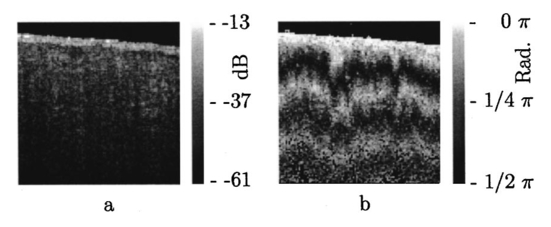

2.4.

Stokes Vector and Coherency Matrix Formalism

The Stokes vector is composed of four elements, I, Q, U, and V (sometimes denoted s₀, s₁, s₂, and s₃ ) and provides a complete description of the light polarization state. I, Q, U, and V can be measured with a photodetector and linear and circular polarizers. Lets call I_t the total light irradiance incident on the detector, I₀°, I₉₀°, I₊₄₅°, and I₋₄₅° the irradiances transmitted by a linear polarizer oriented at an angle of, respectively, 0°, 90°, +45°, and −45° to the horizontal. Let us define also I_rc and I_lc as the irradiances transmitted by a circular polarizer opaque to, respectively, left and right circularly polarized light. Then, the Stokes parameters are defined by

I = I_{t},

Eq. (20)

Q = (I_{0 °} - I_{90 °}),

U = (I_{+ 45 °} - I_{- 45 °}),

V = (I_{rc} - I_{lc}) .

After normalizing the Stokes parameters by the irradiance I, Q describes the amount of light polarized along the horizontal (Q=+1) or vertical (Q=−1) axes, U describes the amount of light polarized along the +45° (U=+1) or −45° (U=−1) directions, and V describes the amount of right (V=+1) or left (V=−1) circularly polarized light. Figure 3 shows the definition of the normalized Stokes parameters with respect to a right handed coordinate system, where we have adopted the definition of a right-handed vibration ellipse (positive V parameter) for a clockwise rotation as viewed by an observer who is looking toward the light source. Positive rotation angles are defined as counter clockwise rotations. For practical reasons the Stokes vector is sometimes represented in the Poincare´ sphere system,²² where it is defined as the vector between the origin of an x-, y-, z -coordinate system and the point defined by (Q,U,V). The ensemble of normalized Stokes vectors with the same degree of polarization (0<P<1) defines a sphere with radius that varies between 0 for natural light and 1 for totally polarized light.

Figure 3

(a) Definition of the Stokes parameters with respect to a right-handed coordinate system. The light is propagation along the positive z axis, i.e., towards the viewer. Q and U describe linear polarizations in frames rotated by 45° with respect to each other. The V parameter describes circular polarized light. (b) Poincare´ sphere representation of the Stokes parameters (adapted from Ref. 22).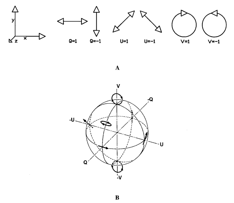

The Poincare´ sphere is a convenient geometrical tool to analyze change in polarization state due to linear, circular, or elliptical birefringence. The transformation of the Stokes vector representing the incident polarization state by a linear retarder is given by a rotation around an axis in the Q–U plane of the Poincare´ sphere. The orientation of the rotation axis corresponds to the orientation of the optic axis with respect to the horizontal. For example, when the optic axis of the linear retarder is at 45° with respect to the horizontal, the rotation axis on the Poincare´ sphere is coincident with the positive U axis. The angle of rotation about the axis on the Poincare´ sphere equals the amount of phase retardation of the linear retarder. From the Poincare´ sphere it is clear that a circular polarization state (V=+/−1) is always perpendicular to a rotation axis in the Q–U plane, and thus will always be modified by a linear retarder, regardless of the orientation of the optic axis. When a linear polarization state is incident parallel to the optic axis of a linear retarder, the state is unchanged. The retardation and orientation of the optic axis of a linear retarder can be determined from the transformation of the Stokes vector in the Poincare´ sphere by finding the three-dimensional rotation matrix with a rotation axis in the Q–U plane that describes the transformation. Circular birefringence (optical activity) is a rotation around the V axis.

For a well collimated, uniform, quasimonochromatic light beam propagating in the z direction with a mean angular frequency ω we can define the electric field components along the x (horizontal) and y (vertical) axes as follows:

Eq. (21)

E_{x} (t) = a_{1} (t) exp {i [α_{1} (t) + ω t]},

E_{y} (t) = a_{2} (t) exp {i [α_{2} (t) + ω t]} .

Then the (non-normalized) Stokes parameters expressed in the variables describing the electric field components can be easily shown to be

I = 〈 a_{1}^{2} 〉 + 〈 a_{2}^{2} 〉,

Eq. (22)

Q = 〈 a_{1}^{2} 〉 - 〈 a_{2}^{2} 〉,

U = 2 〈 a_{1} a_{2} cos [α_{2} (t) - α_{1} (t)] 〉,

V = 2 〈 a_{1} a_{2} sin [α_{2} (t) - α_{1} (t)] 〉 .

Although the Stokes parameters are useful experimentally, the coherency matrix¹⁹ links the polarization state of light more formally to the zero-time correlation properties between orthogonal electric field components. The coherency matrix of a well-collimated, uniform, quasi-monochromatic light beam is defined by¹⁹

Eq. (23)

J = [\begin{matrix} 〈 E_{x}^{*} (t) E_{x} (t) 〉 & 〈 E_{x}^{*} (t) E_{y} (t) 〉 \\ 〈 E_{y}^{*} (t) E_{x} (t) 〉 & 〈 E_{y}^{*} (t) E_{y} (t) 〉 \end{matrix}],

where E_x(t) and E_y(t) are the components of the complex electric field vector along the x and y axes in the plane perpendicular to the light propagation direction. The diagonal elements are real numbers and the off-diagonal elements are complex conjugates. The normalized off-diagonal element is defined as

Eq. (24)

j_{xy} = \frac{J_{xy}}{{(J_{xx})}^{1 / 2} {(J_{yy})}^{1 / 2}}, with 0 \leq | j_{xy} | \leq 1 .

The normalized off-diagonal element |j_xy| is an important parameter and measures the degree of correlation between the x and y field components. The value of |j_xy| is unity for completely polarized light; for partially polarized light 0<|j_xy|<1. Coherency matrix elements and Stokes parameters are related by

Eq. (25)

\begin{matrix} I = J_{xx} + J_{yy} \\ Q = J_{xx} - J_{yy} \\ U = J_{xy} + J_{yx} \\ V = i (J_{yx} - J_{xy}) \end{matrix} \Leftrightarrow \begin{matrix} J_{xx} = \frac{1}{2} (I + Q) \\ J_{yy} = \frac{1}{2} (I - Q) \\ J_{xy} = \frac{1}{2} (U + iV) \\ J_{yx} = \frac{1}{2} (U - iV) \end{matrix} .

Relations in Eq. (25) will be used in the next section to calculate the Stokes parameters from the coherency matrix.

2.5.

Calculating the Stokes Parameters of Reflected Light

Combining the principles of interferometric ellipsometry and OCT, the depth resolved Stokes parameters of reflected light can be determined. As can be seen in Eqs. (13) and (15), the angle α of the sample optic axis with the horizontal gives rise to a phase shift between the interference terms in the horizontal (A_H) and vertical (A_V) polarization channels. The amplitude and relative phase of the interference fringes in each orthogonal polarization channel will be used to derive the depth resolved Stokes vector of reflected light. The use of interferometry to characterize the polarization state of laser light specularly reflected from a sample was apparently first demonstrated by Hazebroek and Holscher.¹¹ In their work, coherent detection of the interference fringe intensity in orthogonal polarization states formed by HeNe laser light in a Michelson interferometer was used to determine the Stokes parameters of light reflected from a sample. Using a source with short temporal coherence adds path length discrimination to the technique, since only light reflected from the sample with an optical path length equal to that in the reference arm within the coherence length of the source will produce interference fringes. When using incoherent detection techniques, only two of the four Stokes parameters can be determined simultaneously. In the present analysis, we demonstrate that coherent detection of the interference fringes in two orthogonal polarization states allows determination of all four Stokes parameters simultaneously. Before giving a mathematical description, the principles underlying calculation of the Stokes vector will be discussed. We assume that the polarization state of light reflected from the reference arm is perfectly linear, at an angle of 45° with the horizontal axis. After the polarizing beam splitter in the detection arm, the horizontal and vertical field components of light in the reference arm will have equal amplitude and phase. Light reflected from the sample will interfere with that from the reference, and the amplitude and relative phase difference of the interference fringes in each polarization channel will be proportional to the amplitude and relative phase difference between horizontal and vertical electric field components of light reflected from the sample arm. The electric field vector of light reflected from the sample arm can be reconstructed by plotting the interference term of the signals on the horizontal and vertical detectors along the x and y axes, respectively. Figure 4 shows a reconstruction of the electric field vector over a trace of 38 μm. The plot does not reflect the actual polarization state reflected from the sample, since the light has made a return pass through the quarter wave plate in the sample arm before being detected. The plot indicates change in polarization state from a linear to an elliptic state as a consequence of tissue birefringence.

Figure 4

Evolution of the electric component of the electromagnetic wave of the reflected light propagating through birefringent mouse muscle. The electric field is reconstructed from the horizontal A_H and vertical A_V polarized components and relative phase of the interference fringes detected in the experimental scheme shown in Figure 1. The displayed section is a small part of a longitudinal scan in the middle of the image shown in Figure 2. Length of the section is 38 μm in a sample with refractive index n=1.4. The beginning of the section shows the reflection from the sample surface modulated by the coherence envelope. The inserts show cross sections of the electric field over a full cycle perpendicular to the propagation direction taken at, respectively, 5.7 and 35.7 μm from the beginning of the section. As can be seen from the inserts the initial polarization state of reflected light is linear along one of the displayed axes, changing to an elliptical polarization state for reflection deeper in the tissue. Reprinted from Ref. 41 with permission of the Optical Society of America.

The Stokes parameters can be determined from the detected interference fringe intensity signals. For instance, if the interference fringes are maximized on one detector, and minimal on the other, the polarization state is linear in either the horizontal or vertical plane, which corresponds to the Stokes parameter Q being one or minus one. If the interference fringes on both detectors are of equal amplitude and in phase, or π out of phase, the polarization state is linear, at 45° with the horizontal or vertical, corresponding to the Stokes parameter U being one or minus one. If the interference fringes on both detectors are of equal amplitude and are exactly π/2 or −π/2 out of phase, the polarization state is circular, corresponding to the Stokes parameter V being one or minus one.

In the mathematical description that follows, the Stokes vector is calculated by Fourier transforming the interference fringes in each channel over a length of approximately the coherence length, and computing the relative phase difference and amplitude of the Fourier components at each wave number. This will give the Stokes vector for each wave number within this length. The Stokes vector of the reflected light is then obtained by summing the Stokes parameters over the spectrum of the source with a weight determined by the power spectral density S(k).

The electric field amplitude of each polarization component is again represented by a complex analytic function, given in Eq. (4), with the conditions given in Eqs. (5) and (6). As derived earlier [Eq. (10)] the light reflected from the reference arm into the detection arm is given by

Eq. (26)

E_{r} (z_{r}) = \frac{1}{2} \int \tilde{e} (k) exp (- 2 {ikz}_{r}) (\begin{matrix} 1 \\ 1 \end{matrix}) dk,

with z_r the reference arm length. The electric field amplitude of light reflected from the sample into the detection arm may be written as

Eq. (27)

E_{s} (z_{s}) = \frac{1}{2} \sqrt{R (z_{s})} \int a (k, z_{s}) \tilde{e} (k) exp (- 2 {ikz}_{s}) dk,

where R(z_s) is a real number representing the reflectivity at depth z_s and the attenuation of the coherent beam by scattering, and a(k,z_s) is a complex valued Jones’ vector that characterizes the amplitude and phase of each light field component with wave number k that was reflected from depth z_s, with,

Eq. (28)

a^{*} (k, z_{s}) a (k, z_{s}) = 1, and a (k, z_{s}) = 0 if k < 0 .

Equation (27) is a generic expression describing reflected light without assumptions about the cause of the polarization state changes in the sample. Following the notation in Mandel and Wolf,¹⁴ the Stokes parameters s₀=I, s₁=Q, s₂=U, and s₃=V of the electric field amplitude E _s(z_s) are given by,

Eq. (29)

s_{j} (z_{s}) = tr [σ_{j} J] = \frac{1}{4} R (z_{s}) \int [a^{*} (k, z_{s}) σ_{j} a (k, z_{s})] S (k) dk,

where the definition of the 2×2 coherency matrix J [Eq. (23)] and the relation between the coherency matrix elements and the Stokes parameters [Eq. (25)] were used. σ₀ is the 2×2 identity matrix and σ₁, σ₂, and σ₃ are the Pauli spin matrices which we take to be [This definition of the Pauli spin matrices differs from the widely accepted definition σ₁=(₁ ⁰ ₀ ¹), σ₂=(_i ⁰ ₀ ⁻ⁱ), σ₃=(₀ ¹ ₋₁ ⁰)].

Eq. (30)

σ_{1} = (\begin{matrix} 1 \\ 0 \end{matrix} \begin{matrix} 0 \\ - 1 \end{matrix}), σ_{2} = (\begin{matrix} 0 \\ 1 \end{matrix} \begin{matrix} 1 \\ 0 \end{matrix}), σ_{3} = (\begin{matrix} 0 \\ - i \end{matrix} \begin{matrix} i \\ 0 \end{matrix}) .

From Eqs. (6), (26), and (27) the interference fringe intensity between light in the sample and reference paths measured by the two detectors is given by

Eq. (31)

I (z_{s}, Δ z) = 2 Re [\begin{matrix} 〈 E_{rx}^{*} (z_{r}) E_{sx} (z_{s}) 〉 \\ 〈 E_{ry}^{*} (z_{r}) E_{sy} (z_{s}) 〉 \end{matrix}] = \frac{1}{4} \sqrt{R (z_{s})} \times \int 2 Re [a (k, z_{s}) exp (- 2 ik Δ z)] S (k) dk

with Δz=z_r−z_s. The Fourier transform of I(z_s,Δz) with respect to Δz is for notational convenience defined as

Eq. (32)

\tilde{I} (z_{s}, 2 k) = \frac{1}{2 π} \int I (z_{s}, Δ z) exp (2 ik Δ z) d Δ z .

Retaining only the components for positive k of the Fourier transform I˜(z_s,2k) gives the complex cross-spectral density function for each polarization component

Eq. (33)

\tilde{I} (z_{s}, 2 k) = \frac{1}{8 π} \sqrt{R (z_{s})} a (k, z_{s}) S (k) for k > 0 .

Using Eq. (33) the Stokes parameters in Eq. (29) can be expressed in terms of I˜(z_s,2k):

Eq. (34)

s_{j} (z_{s}) = {(8 π)}^{2} \int [{\tilde{I}}^{*} (z_{s}, 2 k) σ_{j} \tilde{I} (z_{s}, 2 k)] / S (k) dk .

The Stokes parameters for each pixel in an image can be calculated according to Eq. (34), with the Fourier components I˜(z_s,2k) determined by the Fourier transform of I(z_s,Δz) over Δz intervals on the order of the coherence length of the source light. The power spectral density S(k) in Eq. (34) is given by

Eq. (35)

S (k) = P_{0} \frac{| \tilde{I} (z_{s}, 2 k) |}{\int | \tilde{I} (z_{s}, 2 k) | d k},

with P ₀ the source power. Substituting Eq. (35) into Eq. (34), the Stokes parameters are completely determined by the source power and the Fourier transform of the interference fringes in each polarization channel over an interval Δz around z_s:

Eq. (36)

s_{j} (z_{s}) = \frac{{(8 π)}^{2} \int | \tilde{I} (z_{s}, 2 k) | dk}{P_{0}} \times \int [{\tilde{I}}^{*} (z_{s}, 2 k) σ_{j} \tilde{I} (z_{s}, 2 k)] /| \tilde{I} (z_{s}, 2 k) | dk .

The earlier equation gives the Stokes parameters as measured at the detectors for a single A-line scan. To determine the polarization state of light reflected from the sample, (i.e., before the return pass through the QWP), the Stokes vector computed from Eq. (36) needs to be multiplied by the inverse of the Mueller matrix associated with the QWP in the sample arm, s₀→s₀, s₁→s₃, s₂→s₂, and s₃→−s₁. PS–OCT images of the Stokes parameters are formed by grayscale coding 10 log s₀(z) and the polarization state parameters s₁, s₂, and s₃ normalized on the intensity s₀ from 1 to −1. When applying an incoherent detection technique that does not compute the relative phase between fringes in orthogonal detection channels, only two of the four Stokes parameters ( s₀ and s₃ ) may be determined from a single A-line scan.

2.6.

The Degree of Polarization

The complete characterization of the polarization state of reflected light by means of the Stokes parameters permits the calculation of the degree of polarization P, defined as

Eq. (37)

P = \frac{\sqrt{Q^{2} + U^{2} + V^{2}}}{I} .

For purely polarized light, the degree of polarization is unity, and the Stokes parameters obey the equality I²=Q²+U²+V², while for partially polarized light, the degree of polarization is smaller than unity, leading to I²>Q²+U²+V². In terms of the coherency matrix, the degree of polarization is given by P=tr(J^Pol)/tr(J) where J^Pol is a Hermitian matrix that represents the portion of the full coherency matrix corrresponding to completely polarized light. Natural light, characterized by its incoherent nature, has (by definition) a degree of polarization of zero. An interferometric gating technique such as OCT measures only the light reflected from the sample arm that does interfere with the reference arm light. On first inspection, this suggests that the degree of polarization will always be unity, since only the coherent part of the reflected light is detected.²³ We will demonstrate however, that the degree of polarization can be smaller than unity, and is a function of the interval Δz over which the degree of polarization is calculated. This can be attributed to a variation of the Stokes vector with wavelength.

An input beam with P<1 can be decomposed into purely polarized beams (P=1). After propagation through an optical system, the Stokes parameters of the purely polarized beam components are added to give the Stokes parameters for the original input beam. In Bohren and Huffman’s words: “If two or more quasi-monochromatic beams propagating in the same direction are superposed incoherently, that is to say there is no fixed relationship between the phases of the separate beams, the total irradiance is merely the sum of individual beam irradiances. Because the definition of the Stokes parameters involves only irradiances, it follows that the Stokes parameters of a collection of incoherent sources are additive.” ⁵ Implicit in our analysis is that a broadband OCT source may be viewed as an incoherent superposition of beams with different wave numbers.

The degree of polarization can be analyzed in terms of the off-diagonal element of the coherency matrix. From the expression for the electric field amplitude of light reflected from the sample [Eq. (27)], we may write an expession for the normalized off-diagonal element of the coherency matrix as

Eq. (38)

j_{xy} = \frac{\int a_{x}^{*} (k, z_{s}) a_{y} (k, z_{s}) S (k) dk}{{[\int {| a_{x} (k, z_{s}) |}^{2} S (k) dk]}^{1 / 2} {[\int {| a_{y} (k, z_{s}) |}^{2} S (k) dk]}^{1 / 2}} .

When the polarization state of reflected light is constant over the source spectrum, then a(k,z_s)=a ₀ is constant and |j_xy|=1 so that the degree of polarization is unity (P=1). When the relative magnitude or phase of the complex numbers a_x(k,z_s) and a_y(k,z_s) change over the source spectrum (i.e., the polarization state of reflected light varies over the source spectrum) we may have |j_xy|<1 and the degree of polarization is less than unity (P<1). In general, we note that 0<|j_xy|⩽P⩽1 and |j_xy|=P when 〈|E_x|²−|E_y|²〉=0. ²⁴

A closer look at Eqs. (34) or (36) reveals that the Stokes parameters of each spectral component of the source are determined with a spectral resolution inversely proportional to the Δz interval over which the Fourier transform was taken. Integration over the wave number k sums the Stokes parameters of each spectral component with a weight proportional to the power spectral density, S(k). The larger the Δz interval, the higher the resolution in k space, the more Stokes parameters of incoherently superposed beams are summed. Using the Poincare sphere representation, one can visualize that the magnitude of a sum of Stokes vectors will be greatest if the direction of all components are colinear. When the Stokes parameters of reflected light do not vary over the source spectrum (the polarization state does not vary), the Stokes vectors add colinearly along one direction and the degree of polarization is maximum with a value of unity (note that in our experimental configuration this holds for the input and reference arm beams). When the Stokes parameters vary over the source spectrum, the polarization state of the various spectral components may be viewed as being distributed over the Poincare sphere. Because all components are not colinear, the sum of Stokes parameters over the spectrum gives a degree of polarization (P) necessarily less than unity (P<1).

An alternative argument will lead to the same conclusion. The reconstruction of the electric field vector in Figure 4 shows that the Stokes parameters can be determined over a single cycle of the field, where at each cycle the degree of polarization will be (very close to) unity. The Stokes parameters over an interval Δz are the sum of the Stokes parameters of single cycles of the electric field vector within the interval. The degree of polarization P of the depth resolved Stokes vector will be a function of the interval length (Δz), since Stokes parameters can vary from cycle to cycle.

The reduction of the degree of polarization with increasing depth, that is demonstrated in Figures 5 and 7, can be attibuted to several factors. First, spectral components that may have traveled over different paths with equal lengths through the sample. Second, spectral dependence of the Stokes parameters of light forward or backscattered by (irregularly shaped) particles. Third, presence of multiple scattered light and speckle in the pupil of the sample arm. Fourth, a decrease in the signal to noise ratio. Note that elastic (multiple) scattering does not destroy the coherence of the light in the sense of its ability to interfere with the source light (or the reference arm light). However, spectral phase variations within or between polarization channels may reduce the coherence envelope in a manner similar to the effect of dispersion. Inelastic interactions, such as incoherent Raman scattering or fluorescence, do destroy the coherence and interference with source light is lost.

Figure 5

PS–OCT images of ex vivo rodent muscle, 1 mm×1 mm, pixel size 10 μm×10 μm. From left to right, the Stokes parameter I, normalized parameters Q, U, and V in the sample frame for right circularly polarized incident light, and the degree of polarization P. The gray scale to the right gives the magnitude of signals, 35 dB range for I, from 1 (white) to −1 (black) for Q, U, and V, and from 1 (white) to 0 (black) for P. Reprinted from Ref. 3 with permission of the Optical Society of America.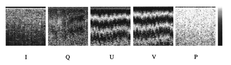

2.7.

Determination of the Optic Axis

Recently, Hitzenberger et al.;²¹ calculated the orientation of the optic axis with a phase sensitive PS–OCT instrument equal to an instrument presented before.³ They determined the phase difference α between the interference fringes in orthogonal polarization channels by use of Hilbert transforms, which gives the orientation of the optic axis [see Eq. (15), and Eq. (2) in Ref. 2] and ignored the amplitude information. However, when the fringe amplitude in one of the two polarization channels is very small (which was the case at the tissue surface in their experimental configuration), it is difficult to extract a reliable phase difference between the two channels. When the optic axis changes with depth, the relative phase difference α becomes uncorrelated with the optic axis orientation. The optic axis orientation can only be determined in the first birefringent layer, where the method suffers the most from a small signal in one of the polarization channels.

The optic axis orientation can be determined more reliably from the Stokes parameters, which uses the amplitude and relative phase difference α.³ This method eliminates the problem associated with determining the relative phase difference between the two polarization channels when the signal at one of the detectors is small compared to the other signal.

To obtain the correct orientation of the optic axis that varies with depth by either method requires a calculation that takes into account the change in the polarization state in previous layers.

A more elaborate description on the determination of the optic axis as presented in Ref. 3 is given here, which assumes the orientation of the optic axis is constant with depth. The values of Q and U depend on the choice of the reference frame (i.e., the orientation of the polarizing beam splitter in the detection arm). The reference frame, or laboratory frame, is determined by the orientation of orthogonal polarization states exiting the polarizing beam splitter, which in our case is along the horizontal and vertical axes. If the basis vectors of the reference frame are rotated through an angle β, the transformation from (I,Q,U,V) to Stokes parameters (I^′,Q^′,U^′,V^′) relative to the new basis vectors is given by⁵

Eq. (39)

(\begin{matrix} I^{'} \\ Q^{'} \\ U^{'} \\ V^{'} \end{matrix}) = (\begin{matrix} 1 & 0 & 0 & 0 \\ 0 & cos 2 β & sin 2 β & 0 \\ 0 & - sin 2 β & cos 2 β & 0 \\ 0 & 0 & 0 & 1 \end{matrix}) (\begin{matrix} I \\ Q \\ U \\ V \end{matrix}) .

The Stokes vector measured in the laboratory frame can be transformed to a new frame, which we will call the sample frame, according to the matrix in Eq. (39).

The Mueller matrix for an ideal retarder is given by⁵

Eq. (40)

(\begin{matrix} 1 & 0 & 0 & 0 \\ 0 & C^{2} + S^{2} cos δ & SC (1 - cos δ) & - S sin δ \\ 0 & SC (1 - cos δ) & S^{2} + C^{2} cos δ & C sin δ \\ 0 & S sin δ & - C sin δ & cos δ \end{matrix}),

where C=cos 2α, S=sin 2α, with α the angle of the optic axis with the horizontal, and δ the retardance. Equation (40) is the Mueller matrix representation of the linear retarder described by the Jones matrix in Eq. (11), with δ=k₀zΔn. Upon specular reflection inside the sample, the Stokes parameters U and V change sign. The angle α of the optic axis of the Mueller matrix for the linear retarder on the return pass changes sign because the coordinate handedness is changed (the propagation direction of the light is reversed). After the return pass through the retarder, the combined Mueller matrix of propagation, reflection, and return pass is given by

Eq. (41)

(\begin{matrix} 1 & 0 & 0 & 0 \\ 0 & C^{2} + S^{2} cos δ & SC (1 - cos δ) & - S sin δ \\ 0 & - SC (1 - cos δ) & - S^{2} - C^{2} cos δ & - C sin δ \\ 0 & - S sin δ & C sin δ & - cos δ \end{matrix}),

with δ=2k₀zΔn. For example, when right circularly polarized light is incident onto a sample with linear retardance, the reflected light polarization state can be defined by the product of the Stokes vector (1,0,0,1) and the above matrix. The reflected light Stokes vector is

Eq. (42)

(\begin{matrix} I \\ Q \\ U \\ V \end{matrix}) = (\begin{matrix} 1 \\ - sin 2 α sin 2 k_{0} z Δ n \\ - cos 2 α sin 2 k_{0} z Δ n \\ - cos (2 k_{0} z Δ n) \end{matrix}) .

From Eq. (42) it is immediately clear that the optic axis orientation α can be determined from the Q and U parameters

Eq. (43)

tan α = Q / U .

Using Eq. (39) to transform the reflected light Stokes vector into a rotated reference frame, we can show that the Q parameter equals 0 if the rotation angle β equals −α. Therefore, the angle of the optic axis is found by determining the angle of rotation of the reference frame that minimizes the amplitude of oscillations with depth in the Q parameter. This angle defines a rotation of the laboratory frame to a sample frame whose basis vectors are aligned with the optic axes of the sample.

2.8.

Depth Resolved Imaging of Stokes Parameters

Rodent muscle was mounted in a chamber filled with saline and covered with a thin glass cover slip to avoid dehydration during measurement. Figure 5 shows images of Stokes parameters in the sample frame for right circularly polarized incident light. Several periods of normalized U and V, cycling back and forth between 1 and −1, are observed in muscle indicating that the sample is birefringent, further demonstrated by the averages of the normalized Stokes parameters over all depth profiles in Figure 6(a). To verify experimentally the orientation of the optical axis computed by rotating the reference frame so as to minimize the amplitude of oscillation in Q, three measurements were performed by replacing the QWP in the sample arm by a half-wave retarder. Light incident on the sample was prepared in three linear polarization states with electric fields parallel, perpendicular, and at an angle of 45° to the experimentally determined optical axis of the birefringent muscle. Figure 6(b) shows the average of the normalized Stokes parameter Q over all depth profiles at the same sample location. The negligible amplitude of oscillation in Q for light polarized parallel and perpendicular to the optical axis verified the experimentally determined orientation. When light is incident at an angle of 45° to the optical axis of the sample, Q oscillates with increasing sample depth as expected for a birefringent sample. The similarity of the reflected intensity for circular, parallel and perpendicular light [shown in Figure 6(c)] indicates that the polarization state changes are not due to dichroism of the muscle fibers. The birefringence Δn was determined by measuring the distance of a full V period, which corresponds to a phase retardation of π=k₀zΔn, giving Δn=1.4×10⁻³. The similarity between PS–OCT images coding for the phase retardation φ(z) and the normalized Stokes parameter V [e.g., Figure 2(b) and Figure 5 V ] is due to the close algebraic relation between the two

Eq. (44)

φ (z) = arctan [\sqrt{\frac{I_{V} (z)}{I_{H} (z)}}], V (z) = cos [2 φ (z)] .

Note that φ(z) gives the single pass phase retardation, φ(z)=kΔnz while V(z) is determined by the double pass phase retardation, V(z)=cos(2kΔnz). Figure 7 shows PS–OCT images of the four Stokes parameters in the laboratory frame for right circularly polarized light incident on in vivo rodent skin. Averages of the normalized Stokes parameters Q, U, and V over all depth profiles [Figure 6(d), after minimizing the oscillations in Q ], indicate oscillations typical of sample birefringence in the first 400 μm. Observed birefringence is attributed to the presence of collagen in skin. Although no preferred orientation of the optical axis is expected in rodent skin, a predominant direction was found at shallow depths. At deeper depths, Q, U, and V approach zero and the light becomes depolarized, which is attributed to multiple scattering and the randomly oriented and changing optical axis over the transversal scan width.

Figure 6

Averages of Stokes parameter I, and normalized parameters Q, U, and V in the sample frame over all depth profiles of, respectively, (a) rodent muscle, right circular incident polarization, (b) rodent muscle, linear incident polarization, parallel, perpendicular, and at 45° with the optical axis, (c) rodent muscle, right circular, parallel and perpendicular incident polarization, (d) in vivo rodent skin, right circular incident polarization. Reprinted from Ref. 3 with permission of the Optical Society of America.

Figure 7

PS–OCT images of in vivo rodent skin, 5 mm×1 mm, pixel size 10 μm×10 μm. From top to bottom, the Stokes parameter I, normalized parameters Q, U, and V in the laboratory frame for right circular polarized incident light, and the degree of polarization P. The magnitude of signals ranged over 40 dB for I, from 1 (white) to −1 (black) for Q, U, and V, and from 1 (white) to 0 (black) for P. Reprinted from Ref. 3 with permission of the Optical Society of America.

2.9.

Polarization Diversity Detection

To summarize, PS–OCT is important not only to measure birefringence, but also for accurate interpretation of OCT images. Most fibrous structures in tissue (e.g., muscle, nerve fibers) are form birefringent due to their structural anisotropy. Single detector OCT systems can generate images that show structural properties by a reduction in tissue, reflectivity, solely due to polarization effects. Polarization diversity detection is defined as the depth resolved measurement of the I component of the Stokes vector of light reflected from the sample. Intuitively, one might expect that use of unpolarized sources may be advantageous for polarization diversity detection.

Although the source light has been assumed to be polarized, the presented analysis is easily extended to include unpolarized sources. An unpolarized source can be described by the addition of two orthogonally polarized sources that are mutually incoherent. The interference fringes at the detector(s) need to be analyzed separately for the two pure polarization states and the total interference fringe pattern at the detector(s) is given by the sum of the fringe patterns of each polarization channel.

An OCT system with an unpolarized source and a single detector does not necessarily provide polarization diversity detection. On the contrary, this system can be more sensitive to polarization effects than a system with a polarized source.

Consider polarized source light incident on a birefringent sample acting as linear retarder with optic axis at 45° with respect to the incident light polarization axis. The polarization state of reflected light from some depth has undergone a π phase retardation and is orthogonal to the incident polarization state. Since orthogonally polarized states cannot interfere, light from the sample and reference arms do not produce interference fringes. The same holds for each of the orthogonally polarized states in the decomposition of an unpolarized source into linear states at 45 and −45 with the optic axis. Therefore, for the unpolarized source no interference fringes will be detected. Suppose now that the decomposition of the unpolarized source is chosen differently for the earlier mentioned birefringent sample, such that the two orthogonal linearly polarized mutually incoherent states are along and perpendicular to the optic axis. Both orthogonal polarization states reflected from the sample are unaltered by the birefringence, and will produce interference fringes with the reference arm light. However, at the same depth as above the interference fringes for orthogonal polarization states are exactly π out of phase and cancel after summation on the single detector, and no interference fringe pattern is observed. Thus, in this example, the unpolarized source will not produce interference fringes at one depth regardless of the orientation of the optic axis (as is expected from symmetry arguments). In contrast, a polarized source would produce interference fringes if the state is polarized (partially) along the optic axis.

2.10.

Accuracy and Noise; Birefringence, Dichroism and Scattering

Everett et al.;¹⁵ have given an analysis of the systematic error in the phase retardation due to background noise for the incoherent PS–OCT detection scheme. They showed that for phase retardations close to 0° or 90° the background noise on the detectors introduces a significant and systematic error of, e.g., 15° at a signal to noise ratio of 10 dB. The coherent detection scheme which calculates the Stokes parameters, has better immunity to this systematic error. A closer look at Eqs. (25), (34), or (36) reveals that in the calculation of the Q parameter (also denoted by s₁ ) the spectral density in one polarization channel is subtracted from the spectral density in the orthogonal polarization channel, thus eliminating constant background noise terms, and the U (s₂) and V (s₃) parameters are calculated from the cross correlation between fringes in orthogonally polarized channels, eliminating autocorrelation noise. Noise will decrease the degree of polarization P, since it will be present as autocorrelation noise in the Stokes parameter I. The better noise immunity can be illustrated with the help of Figure 6(a), which shows the Stokes parameters for rodent muscle. In the incoherent detection scheme only V ( s₃ in the figure) is measured, and the error in the phase retardation is introduced by the decrease of the amplitude of oscillations with increasing depth. In the coherent detection scheme, the Stokes parameters Q, U, and V can be renormalized on P, restoring the amplitude of the oscillations, and thus eliminating the systematic error.

Schoenenberger et al.;²⁰ have gone further and also analyzed system errors introduced by the extinction ratio of polarizing optics and chromatic dependence of wave retarders, and errors due to dichroism, i.e., the differences in the absorption and scattering coefficients for polarized light in tissue. System errors can be kept small by careful design of the system with achromatic elements, but can never be completely eliminated. Dichroism is a more serious problem when interpreting the results as solely due to birefringence. However, Mueller matrix ellipsometry measurements have shown that the error due to dichroism in the eye is relatively small²⁵ ²⁶ and Figure 6(c) shows that dichroism is of minor importance in rodent muscle. More research is necessary to determine the importance of dichroism in other types of tissue.

The variance in the computed Stokes vectors of reflected light (excluding effect of birefringence) is due to multiple scattering, speckle, and shot noise (i.e., optimized system). At some depth, the detected signals are limited by shot noise. At shallower depths (i.e., before the shot noise limit) variance in the Stokes parameters is primarily due to the effects of multiple scattering and speckle.

As argued earlier, multiple scattering will scramble the polarization mainly in a random manner. This offers some means to distinguish it from birefringence. Reported birefringence values for cornea, tendon, and muscle are of the order of Δn=10⁻³, ²⁷ ²⁸ ²⁹ which will give a 90° phase retardation at a depth on the order of several hundreds of micrometers. Thus, birefringence induced changes are relatively slow, and the Stokes parameters change according to the Mueller matrix of a linear retarder. However, an optic axis that varies with depth will give changes in the polarization state that will be difficult to distinguish from the random manner of multiple scattering. Measurement of the full Mueller matrix of the sample by varying the incident light over four different polarization states, as recently demonstrated by Yao and Wang,³⁰ will provide additional information that could aid the analysis and interpretation of PS–OCT signals. More research is necessary on this complex problem.

Speckle introduces noise on the Stokes parameters by the large fluctuations in the interference fringes that could be uncorrelated in the orthogonal detection channels. Speckle averaging techniques demonstrated by Schmitt et al.;³¹ will reduce this noise, as well as averaging the Stokes parameters over distances larger than the coherence length. Speckle remains one of principle problems in the development of OCT.

3. Future Directions in PS–OCT

Investigation of the biological and medical applications of PS–OCT is just beginning and much work remains for further development. We anticipate progress will proceed in three major areas, these include: instrumentation, biological and medical applications, and data interpretation/image processing. Many investigators have reported use of a bulk polarization-sensitive interferometer for imaging biological materials.¹⁴ ¹⁵ ³⁰ ³² ³³ Work by Yao and Wang³⁰ and Jiao and Wang³⁴ is noteworthy in that the depth-resolved Mueller matrix of light reflected from a sample was estimated.

More recently, several groups have reported application of polarization sensitive OCT for biomedical imaging³⁵ ³⁶ ³⁷ using fiber interferometers. Although systems constructed of conventional single mode fiber can maintain a pure polarization state incident on the sample, the state fluctuates in time due to stress perturbations in the fiber. Despite the fluctuation, depth resolved phase retardation of light reflected from the sample is determined by systematically varying the incident polarization state between orthogonal points on the Poincare´ sphere positioned on a great circle.³⁵ Although systems constructed of polarization maintaining single mode fiber can maintain a fixed polarization state incident on the sample, experimental demonstration of such a system that measures the depth-resolved Stokes parameters of reflected light has not been reported.

Because many components in biological materials contain intrinsic and/or form birefringence, PS–OCT is an attractive technique for providing an additional contrast mechanism that can be used to image/identify structural components. For example, recent application of PS–OCT in dentistry,³⁸ ³³ ophthalmology,³² ³⁹ and dermatology³ ³⁵ ⁴⁰ has been reported. Moreover, because functional information in some biological systems is associated with transient changes in birefringence, the possibility of functional PS–OCT imaging should be explored. PS–OCT may hold considerable potential for monitoring, in real-time, laser surgical procedures involving birefringent biological materials. Because many laser surgical procedures rely on a photothermal injury mechanism, birefringence changes in subsurface tissue components measured using PS–OCT may be used as a feedback signal to control laser dosimetry in real-time. Finally, many features of PS–OCT interference fringe data require additional interpretation and study. Because polarization changes in light propagating in the sample may be used as an additional contrast mechanism, the relative contribution of light scattering and birefringence-induced changes requires further study and clarification. In principle, one would like to distinguish polarization changes due to scattering, form and intrinsic birefringence at each position in the sample and utilize each as a potential contrast mechanism. Better distinction between sources of the polarization changes will allow application of various image processing algorithms (e.g., segmentation) that can improve usability of PS–OCT for specific applications. In summary, we expect PS–OCT will continue to advance rapidly and be applied to novel problems in clinical medicine and biological research.

Acknowledgments

Research grants from the Institute of Arthritis, Musculoskeletal and Skin Diseases, and Heart, Lung and Blood, and the Eye Institute, and the National Center for Research Resources at the National Institutes of Health, U.S. Department of Energy, Office of Naval Research, the Whitaker Foundation (26083), and the Beckman Laser Institute Endowment are gratefully acknowledged.

REFERENCES

1.

D. Huang , E. A. Swanson , C. P. Lin , J. S. Schuman , W. G. Stinson , W. Chang , M. R. Hee , T. Flotte , K. Gregory , C. A. Pufialito , and J. G. Fujimoto , “Optical coherence tomography,” Science , 254 1178 –1181 (1991). Google Scholar

2.

J. F. de Boer , T. E. Milner , M. J. C. van Gemert , and J. S. Nelson , “Two-dimensional birefringence imaging in biological tissue by polarization-sensitive optical coherence tomography,” Opt. Lett. , 22 934 –936 (1997). Google Scholar

3.

J. F. de Boer , T. E. Milner , and J. S. Nelson , “Determination of the depth resolved Stokes parameters of light backscattered from turbid media using polarization sensitive optical coherence tomography,” Opt. Lett. , 24 300 –302 (1999). Google Scholar

4.

G. Mie , “Beitrage zur optik tru¨ber medien speziell kolloidaler metallo¨sungen,” Ann. Phys. (Leipzig) , 25 377 (1908). Google Scholar

5.

C. F. Bohren and D. R. Huffman, Absorption and Scattering of Light by Small Particles, Wiley, New York (1983).

6.

W. S. Bickle and W. B. Bailey , “Stokes vectors, Mueller matrices, and polarized light scattered light,” Am. J. Phys. , 53 (5), 468 –478 (1985). Google Scholar

7.

M. I. Mishchenko and J. W. Hovenier , “Depolarization of light backscattered by randomly oriented nonspherical particles,” Opt. Lett. , 20 1356 –1358 (1995). Google Scholar

8.

C. Brosseau, Fundamentals of Polarized Light: A Statistical Optics Approach, Wiley, New York (1998).

9.

E. Collet, Polarized Light: Fundamentals and Applications, Marcel Dekker, New York (1993).

10.

M. Henry , “Fresnel–Arago laws for interference in polarized light: A demonstration experiment,” Am. J. Phys. , 49 690 –691 (1981). Google Scholar

11.

H. F. Hazebroek and A. A. Holscher , “Interferometric ellipsometry,” J. Phys. E , 6 822 –826 (1973). Google Scholar

12.

T. P. Newson , F. Farahi , J. D. C. Jones , and D. A. Jackson , “Combined interferometric and polarimetric fiber optic temperature sensor with a short coherence length source,” Opt. Commun. , 68 161 –165 (1988). Google Scholar

13.

M. Kobayashi , H. Hanafusa , K. Takada , and J. Noda , “Polarization-independent interferometric optical-time-doamin reflectometer,” J. Lightwave Technol. , 9 623 –628 (1991). Google Scholar

14.

M. R. Hee , D. Huang , E. A. Swanson , and J. G. Fujimoto , “Polarization-sensitive low-coherence reflectometer for birefringence characterization and ranging,” J. Opt. Soc. Am. B , 9 903 –908 (1992). Google Scholar

15.

M. J. Everett , K. Schoenenberger , B. W. Colston Jr. , and L. B. Da Silva , “Birefringence characterization of biological tissue by use of optical coherence tomography,” Opt. Lett. , 23 228 –230 (1998). Google Scholar

16.

W. H. Steel , “Two-beam interferometry,” Prog. Opt. , 5 147 –197 (1966). Google Scholar

17.

E. Bernabeu and L. L. Sanchez-Soto , “Coherency matrix analysis of polarization effects in two-beam interferometers,” Optik (Stuttgart) , 74 134 –139 (1986). Google Scholar

18.

R. Barakat , “Theory of the coherency matrix for light of arbitrary spectral bandwidth,” J. Opt. Soc. Am. , 53 317 –323 (1963). Google Scholar

19.

L. Mandel and E. Wolf, Optical Coherence and Quantum Optics, Cambridge University Press, Cambridge (1995).

20.

K. Schoenenberger , B. W. Colston Jr. , D. J. Maitland , L. B. Da Silva , and M. J. Everett , “Mapping of birefringence and thermal damage in tissue by use of polarization-sensitive optical coherence tomography,” Appl. Opt. , 37 6026 –6036 (1998). Google Scholar

21.

C. K. Hitzenberger , E. Gotzinger , M. Sticker , M. Pircher , and A. F. Fercher , “Measurement and imaging of birefringence and optic axis orientation by phase resolved polarization sensitive optical coherence tomography,” Opt. Express , 9 780 –790 (2001). Google Scholar

22.

W. A. Shurcliff and S. S. Ballard, Polarized Light, Van Nostrand, Princeton (1964).

23.

S. Jiao , G. Yao , and L. V. Wang , “Depth-resolved two-dimensional Stokes vectors of backscattered light and Mueller matrices of biological tissue measured with optical coherence tomography,” Appl. Opt. , 39 6318 –6324 (2000). Google Scholar

24.

M. Born and E. Wolf, Principles of Optics, 7th ed., p. 629, Cambridge University Press, Cambridge (1999).

25.

G. J. van Blokland , “Ellipsometry of the human retina in vivo: preservation of polarization,” J. Opt. Soc. Am. A , 2 72 –75 (1985). Google Scholar

26.

H. B. Klein Brink and G. J. van Blokland , “Birefringence of the human foveal area assessed in vivo with Mueller-matrix ellipsometry,” J. Opt. Soc. Am. A , 5 49 –57 (1988). Google Scholar

27.

E. J. Naylor , “The structure of the cornea as revealed by polarized light,” Q. J. Microsc. Sci. , 94 83 –88 (1953). Google Scholar

28.

E. P. Chang , D. A. Keedy , and C. W. Chien , “Ultrastructures of rabbit corneal stroma: Mapping of optical and morphological anisotropies,” Biochim. Biophys. Acta , 343 615 –626 (1974). Google Scholar

29.

D. J. Maitland and J. T. Walsh , “Quantitative measurements of linear birefringence during heating of native collagen,” Lasers Surg. Med. , 20 310 –318 (1997). Google Scholar

30.

G. Yao and L. Wang , “Two-dimensional depth-resolved Mueller matrix characterization of biological tissue by optical coherence tomography,” Opt. Lett. , 24 537 –539 (1999). Google Scholar

31.

J. M. Schmitt , “Array detection for speckle reduction in optical coherence microscopy,” Phys. Med. Biol. , 42 1427 –1439 (1997). Google Scholar

32.

M. G. Ducros , J. F. de Boer , H. Huang , L. Chao , Z. Chen , J. S. Nelson , T. E. Milner , and H. G. Rylander , “Polarization sensitive optical coherence tomography of the rabbit eye,” IEEE J. Sel. Top. Quantum Electron. , 5 1159 –1167 (1999). Google Scholar

33.

A. Baumgartner , S. Dichtl , C. K. Hitzenberger , H. Sattmann , B. Robl , A. Moritz , A. F. Fercher , and W. Sperr , “Polarization-sensitive optical coherence tomography of dental structures,” Caries Res. , 34 (1), 59 –69 (2000). Google Scholar

34.

S. Jiao and L. V. Wang , “Two-dimensional depth-resolved Mueller matrix of biological tissue measured with double-beam polarization-sensitive optical coherence tomography,” Opt. Lett. , 27 101 –103 (2002). Google Scholar

35.

C. E. Saxer , J. F. de Boer , B. H. Park , Y. Zhao , C. Chen , and J. S. Nelson , “High speed fiber based polarization sensitive optical coherence tomography of in vivo human skin,” Opt. Lett. , 25 1355 –1357 (2000). Google Scholar

36.

J. E. Roth , J. A. Kozak , S. Yazdanfar , A. M. Rollins , and J. A. Izatt , “Simplified method for polarization-sensitive optical Coherence tomography,” Opt. Lett. , 26 1069 –1071 (2001). Google Scholar

37.

D. Dave´ and T. E. Milner , “Doppler angle measurement in highly scattering media,” Opt. Lett. , 25 1523 –1525 (2000). Google Scholar

38.

X. J. Wang , T. E. Milner , J. F. deBoer , Y. Zhang , D. H. Pashley , and J. S. Nelson , “Characterization of dentin and enamel by use of optical coherence tomography,” Appl. Opt. , 38 2092 –2096 (1999). Google Scholar

39.

M. D. Ducros , J. D. Marsack , H. G. Rylander III , S. L. Thomsen , and T. E. Milner , “Primate retina imaging with polarization-sensitive optical coherence tomography,” J. Opt. Soc. Am. A , 18 2945 –2956 (2001). Google Scholar

40.

B. H. Park , C. Saxer , S. M. Srinivas , J. S. Nelson , and J. F. de Boer , “In vivo burn depth determination by high-speed fiber-based polarization sensitive optical coherence tomography,” J. Biomed. Opt. , 6 474 –479 (2001). Google Scholar

41.

J. F. de Boer, T. E. Milner, and J. S. Nelson, “Two dimensional birefringence imaging in biological tissue using phase and polarization sensitive optical coherence tomography,” in Advances in Optical Imaging and Photon Migration, Trends in Optics and Photonics (TOPS) Vol. 21, J. G. Fujimoto and M. S. Patterson, Eds., pp. 321–324, Optical Society of America, Washington, DC (1998).

Citation Download Citation

Johannes F. de Boer and Thomas E. Milner "Review of polarization sensitive optical coherence tomography and Stokes vector determination," Journal of Biomedical Optics 7(3), (1 July 2002). https://doi.org/10.1117/1.1483879

Published: 1 July 2002

Access the abstract

JOURNAL ARTICLE
13 PAGES

DOWNLOAD PAPER SAVE TO MY LIBRARY