Near-infrared imaging in the small animal brain: optimization of fiber positions

Heng Xu; Hamid Dehghani; Brian W. Pogue; Roger Springett; Keith D. Paulsen; Jeff F. Dunn

doi:10.1117/1.1528597

1 January 2003 Near-infrared imaging in the small animal brain: optimization of fiber positions

Heng Xu, Hamid Dehghani, Brian W. Pogue, Roger Springett, Keith D. Paulsen, Jeff F. Dunn

Author Affiliations +

Journal of Biomedical Optics, Vol. 8, Issue 1, (January 2003). https://doi.org/10.1117/1.1528597

1. Introduction

Near-infrared (NIR) tomography is a method for imaging biological tissue that has been developing over the past decade.¹ ² ³ ⁴ It has been widely accepted that near-infrared spectroscopy (NIRS) offers a way to noninvasively quantify and monitor changes in tissue hemoglobin concentration and oxygen saturation simultaneously, as well as several other chromophores, such as water, lipids, and cytochrome-c-oxidase. The ability to noninvasively quantify these chromophores is important for understanding physiological function and pathophysiological changes within tissue.⁵ ⁶ However, NIRS imaging traditionally suffers from poor spatial resolution in comparison to other imaging modalities such as magnetic resonance imaging (MRI), owing to the diffuse path of light travel through tissue. In contrast, MRI is able to detect blood oxygen level (BOLD) with millimeter spatial resolution, but its use is limited to well-characterized situations where the physiological interpretation is straightforward.⁷ ⁸ ⁹ Therefore, it is natural to consider combining the merits of MRI with NIRS. Furthermore, by using the high resolution provided by MRI as a prior knowledge, it may be possible to achieve significant improvement in resolution and accuracy of NIR images.¹⁰ ¹¹ ¹²

The data collection and reconstruction of NIR tomographic images involves significant design considerations, many of which are related to the expected field of view. This work concentrates on images in the range of 2 to 4 cm in diameter, to focus on the study of murine models of disease. It includes investigations of metabolic, stroke, and tumor models in rats and transgenic mice. The NIR system being developed will be used to study cerebral oxygenation in infarcts and tumors or in hypoxia/ischemia sensitive regions of the brain such as the hippocampus. A number of groups have previously worked on near-infrared diffuse tomography with a priori MRI structural information, including ourselves.¹⁰ ¹¹ ¹² ¹³ In our earlier studies, a hybrid image reconstruction method was tested in the context of functional imaging of the rat cranium.¹⁰ ¹¹ We used eight separate source and detector fibers located in a circular tomographic array equally spaced around the head of the animal, which produced an image with the brain situated toward the edge [at the left of the cross-sectional image of the head in Figure 1(a)]. Since the brain of the rat was not in the center of the fiber array, it may be possible to optimize the optical source and detector fiber placement to improve sensitivity and resolution in the brain itself.

Figure 1

(a) MRI image of the rat brain used for segmentation of structures within the model. To more precisely locate the external surface of the rat, the animal was enveloped in wet paper towels (which appear as a thick bright band around the animal). (b) The FEM mesh generated from the segmented data with equally spaced optical fibers on the periphery, and (c) optical fibers arranged near the brain and one on the opposite side. The circular black dots represent each of the source optical fibers mounted on the surface and the diamonds represent each of the optical fiber detectors.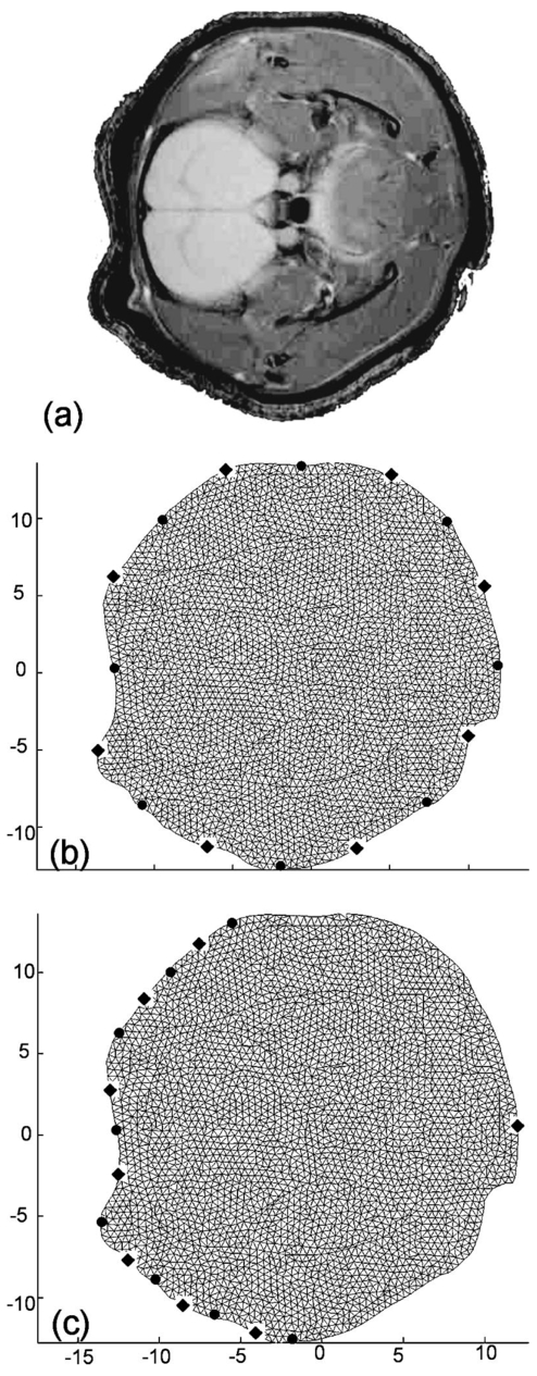

Culver et al.;¹⁴ showed that singular value decomposition analysis could be used to optimize detector placement in the reflectance and direct transmittance geometries of a homogeneous medium, and indicated that this could be extended to arbitrary geometries with heterogeneous tissue volumes. In the present work, the effects of grouping the optical fibers at the top of the skull versus spacing them in a circle around the cranium are investigated to help determine the optimum position with respect to providing information from the brain. The development makes use of a priori structure obtained from MRI scans of the rat head and segmentation of the interior tissue volumes of interest. The propagation of light through scattering tissue can be modeled using the diffusion approximation (DA). Furthermore, for a given source and detector combination, functions are calculated that describe the sensitivity of each source and measurement pair to changes in optical properties (absorption μ_a and scatter μ_s ^′) within each pixel of the model. The inversion of the sensitivity matrix therefore provides a reconstruction of the properties. The singular value analysis of this sensitivity matrix can be used to determine the fraction of information that is higher than the measurement noise level in the typical detection system.

In this work, it has been hypothesized that placing the optical fibers on the side of the head nearest to the brain is equivalent to or better than arranging them equally spaced around the entire head for maximizing sensitivity of the brain tissue to measured data. The arc of fibers around the region of the brain should provide better coverage and allow better resolution of absorption changes within the brain. This hypothesis is tested by evaluating the sensitivity maps of two different optical fiber configurations and using singular value analysis of these maps to calculate the amount of information contained in each set of measurements. The sensitivity maps of the region of interest, the brain, are extracted, and the singular values for each source-detector configuration are calculated and compared. Further, the two different arrangements of optical fibers are used to investigate image reconstruction in the presence of an absorbing anomaly within the brain. The presence of structure within the head is also examined to see if there exist any underlying effects in our analysis from the existence of tissue layers.

2. Methods

A Sprague Dawley rat was imaged using a 7 T horizontal-bore nuclear magnetic resonance system with a Varian Unity console. T2 weighted (TR/TE=1/0.03 s) data was used to obtain structural images of the rat head, and one such slice is shown in Figure 1(a). The image is 256×512 voxels representing a 35×35 mm field of view. Based on this image, the head was segmented to regions of skull, brain, muscle, and skin. From these segmented regions a two-dimensional mesh of the head was generated, as shown in Figure 1(b) and 1(c). Each region was then assumed to have homogeneous and isotropic optical properties and was assigned different optical properties, using values listed in Table 1. This type of prior knowledge about brain structure helps accurate modeling and image reconstruction from measured NIR data, and provides a realistic simulation volume in which to test the hypothesis of this work.

Table 1

Optical properties for each tissue within the FEM model. Rat brain tissue optical properties are based upon measurements by Cope and Delpy.19 Optical properties of skull bone are based upon measurements by Firbank et al.;20 Optical properties of skin and muscle come from Simpson et al.;2122
Region	μ_a (mm⁻¹)	μ_s ^′ (mm⁻¹)
Skin	0.036	1.48
Skull	0.054	0.63
Muscle	0.05	1.46
Brain	0.046	1.95

A finite-element model is used as a general and flexible method for solving the forward problem in arbitrary geometries. Light propagation through tissue can be calculated by application of the diffusion approximation to our model²:

Eq. (1)

- \nabla \cdot κ (r) \nabla Φ (r, ω) + (μ_{a} + \frac{i ω}{c}) Φ (r, ω) = q_{0} (r, ω)

where q₀(r,ω) is an isotropic source, Φ(r,ω) is the photon density at position r and frequency ω, and κ=1/[3×(μ_a+μ_s ^′)] is the diffusion coefficient, where μ_a and μ_s ^′ are the probabilities per unit length of absorption and transport scattering, respectively. We use the Robin-type (type III) boundary condition:

Eq. (2)

Φ (γ) + \frac{κ}{α} \hat{n} \cdot \nabla Φ (γ) = 0,

where α is a term that incorporates reflection as a result of refractive index mismatch at the boundary¹⁵ and n^ is the outer normal to the boundary at γ. This study uses a frequency domain system, and so for an oscillating source input of light the phase and amplitude of the exiting data are measured at positions along the tissue surface (also called boundary data). This phase and amplitude of boundary data depend on the geometry of the region under investigation as well the optical absorption and scatter of the associated tissues. Two different configurations of optical fiber placement are examined in this study, as shown by the pictorial locations of the sources and detectors in Figures 1(b) and 1(c).

A sensitivity map (the Jacobian) was calculated, which related the change in the boundary data (either amplitude or phase) with respect to a small change in either μ_a or κ. The Jacobian maps the optical properties of tissue onto the measurements. This function essentially contains numerical values associated with each node of the model that are proportional to the log of amplitude and phase of light propagation between each source and detector combinations. In our study, the Jacobian matrix J is calculated using the Adjoint method¹⁶ and it has the form

Eq. (3)

J = | \begin{matrix} \frac{δ ln I_{1}}{δ κ_{1}} & \frac{δ ln I_{1}}{δ κ_{2}} & \dots & \frac{δ ln I_{1}}{δ κ_{N}} & ; & \frac{δ ln I_{1}}{δ μ_{a 1}} & \frac{δ ln I_{1}}{δ μ_{a 2}} & \dots & \frac{δ ln I_{1}}{δ μ_{aN}} \\ \frac{δ θ_{1}}{δ κ_{1}} & \frac{δ θ_{1}}{δ κ_{2}} & \dots & \frac{δ θ_{1}}{δ κ_{N}} & ; & \frac{δ θ_{1}}{δ μ_{a 1}} & \frac{δ θ_{1}}{δ μ_{a 2}} & \dots & \frac{δ θ_{1}}{δ μ_{aN}} \\ \frac{δ ln I_{2}}{δ κ_{1}} & \frac{δ ln I_{2}}{δ κ_{2}} & \dots & \frac{δ ln I_{2}}{δ κ_{N}} & ; & \frac{δ ln I_{2}}{δ μ_{a 1}} & \frac{δ ln I_{2}}{δ μ_{a 2}} & \dots & \frac{δ ln I_{2}}{δ μ_{aN}} \\ \frac{δ θ_{2}}{δ κ_{1}} & \frac{δ θ_{2}}{δ κ_{2}} & \dots & \frac{δ θ_{2}}{δ κ_{N}} & ; & \frac{δ θ_{2}}{δ μ_{a 1}} & \frac{δ θ_{2}}{δ μ_{a 2}} & \dots & \frac{δ θ_{2}}{δ μ_{aN}} \\ ⋮ & ⋮ & ⋱ & ⋮ & ⋮ & ⋮ & ⋮ & ⋱ & ⋮ \\ \frac{δ ln I_{M}}{δ κ_{1}} & \frac{δ ln I_{M}}{δ κ_{2}} & \dots & \frac{δ ln I_{M}}{δ κ_{N}} & ; & \frac{δ ln I_{M}}{δ μ_{a 1}} & \frac{δ ln I_{M}}{δ μ_{a 2}} & \dots & \frac{δ ln I_{M}}{δ μ_{aN}} \\ \frac{δ θ_{M}}{δ κ_{1}} & \frac{δ θ_{M}}{δ κ_{2}} & \dots & \frac{δ θ_{M}}{δ κ_{N}} & ; & \frac{δ θ_{M}}{δ μ_{a 1}} & \frac{δ θ_{M}}{δ μ_{a 2}} & \dots & \frac{δ θ_{M}}{δ μ_{aN}} \end{matrix} |,

where δ ln I_i/δκ_j, δ ln I_i/δμ_aj are the submatrices that define the relation between the log of the amplitude of the i’th measurement with respect to κ and μ_a at the j’th reconstructed nodes, respectively, δθ_i/δκ_j, δθ_i/δμ_aj are the submatrices that define the relation between the phase of the i’th measurement with respect to κ and μ_a at the j’th reconstructed nodes, respectively, M is the total number of measurements, and N is the total number of nodes. These four submatrices can be looked at as four types of sensitivity map. Examples of individual rows in the Jacobian matrix plotted as images are shown in Figure 2 (see Color Plate 1), where these sensitivity maps have been calculated on a model of the rat head containing multiple layers of tissue with varying optical properties (properties as listed in Table 1). These maps relate a small change in the log amplitude of the boundary data for a given source detector pair, due to a small change only in optical absorption at all pixel locations. Figure 2 shows that for certain source and detector pairs the brain region is sensitive, with the pair in Figure 2(a) showing more sensitivity than the pair in Figure 2(b). The image in Figure 2(c) shows that the data for some source-detector pairs are substantially less sensitive to the brain, since the optical path between this source-detector pair almost does not go through the brain region. Similar maps can be calculated for other data types (phase of the measured signal) and optical parameters (diffusion coefficient κ). It is important to note that these sensitivity maps are calculated for a model that includes a priori knowledge about the structure and optical properties of all regions in the head. If it were assumed, incorrectly, that the model is homogeneous and therefore these maps are calculated for a homogeneous medium, a different and incorrect sensitivity map would result. Iterative reconstruction of the internal optical properties requires that these sensitivity maps are initially calculated with an initial estimate of the optical properties, but then that they are updated at each iteration step, thereby making the final reconstruction more accurate.

Figure 2

The sensitivity maps (log amplitude of data and μ_a) for three pairs of source and detector positions. In each image, S shows the position of the source, and D the position of the detector.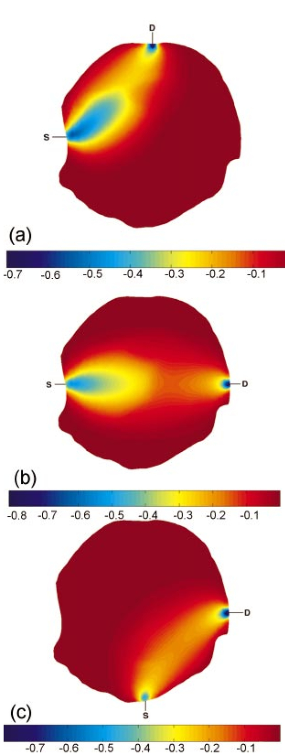

The major focus of this study has been to investigate the effect of different arrangements of the sources and detectors, and the amount of information that can be obtained from these measurements. Culver et al.;¹⁴ have discussed that the magnitude of the singular values of the Jacobian (the weight matrix in their paper) provides a measure of the relative effects of changes in a given region of interest on the detected signal. Here, our Jacobian matrix is the same as the weight matrix. Singular values decomposition of the Jacobian matrix yields a triplet of matrices:

Eq. (4)

J = {USV}^{T},

where U and V are orthonormal matrices containing the singular vectors of J and S is a diagonal matrix containing the singular values of J. Since J helps to map measurements onto optical properties, it can be looked at as an interface between the detection space and the image space. Furthermore, the vectors of U and V correspond to the modes in the detection space and image space, respectively, while the magnitude of singular values in S represents the importance of the corresponding singular vectors in U and V. More nonzero singular values and more modes are effective in two spaces, which bring more details and improve the resolution in the space. In a practical setup, noise should be considered, since this means that only the singular values larger than the noise level could provide useful information. The singular values of the sensitivity maps for the region of interest for a given data type and optical properties (i.e., the brain, using log of amplitude of signal and changes in μ_a) are calculated. There are normally M nonzero singular values in the diagonal matrix when N is larger than M and those values are sorted in decreasing order. Thus, it is possible to determine whether an identical amount of information can be obtained for a change in μ_a within the brain for various configurations of optical fibers. First, the equally spaced arrangement was considered [configuration 1, shown in Figure 1(b)] and second the optical fibers were concentrated over the surface of the head nearest to the brain and another on the opposite side [configuration 2, in Figure 1(c)]. These two configurations were chosen because equally spaced optical fibers are the most conventional arrangement for unbiased sampling of a circular domain, whereas incorporating knowledge of the location of the brain might lead to the argument that the fibers should be concentrated more locally around the brain. Here, there are eight pairs of source and detector fibers, Figure 1(b), spaced equally along the arc of tissue overlying the brain. In this study, the practical number of fibers is chosen by the hardware of the detection system, which is eight sources and eight detectors. Therefore, the number of measurements would be 64. The positioning of fibers near the side of the head in which the brain is located represents a higher density of measurements per unit volume over the tissue surface, and so would suggest that higher spatial resolution should be obtained. A single measurement fiber located on the opposite side, Figure 1(c), provides additional information from the lower portion of the brain in transmittance geometry. The need for this fiber also has been tested and it showed that if the fiber is removed, the reconstruction is not as good as when the fiber is included.

Two separate cases of optical property distribution were considered. The first is a homogeneous case [see Figure 3(a) (color plate 1)], where all elements are assigned the same optical properties (that of the brain alone, where μ_a=0.046 mm ⁻¹ and μ_s ^′=1.95 mm ⁻¹) . Second is the layered model [see Figure 3(b)], where the elements are assigned with the optical properties that correspond to the layer in which they belong. Optical properties for that model are shown in Table 1. The sensitivity maps throughout the model for each data type and optical property (log of amplitude, phase, μ_a, and μ_s ^′) are calculated. From these maps the sensitivity of the data to changes in the brain is only of interest. With this in mind, the sensitivity of this region is extracted from the whole map, using a priori information about the location of the brain. From these isolated sensitivity maps of the brain region, a singular value analysis is performed showing the amount of information that is available from each optical fiber arrangement that corresponds to only the brain region.

Figure 3

The FEM meshes: (a) the homogeneous case, i.e., only one layer, optical properties chosen to be that of the brain alone, and (b) the layered case, i.e., skin, muscle, skull, and brain layer all are added, with each having optical properties shown in Table 1.

Beyond the increase in singular values for a given noise level, the influence of the two optical fiber configurations on the ability of our reconstruction algorithm to resolve a small change in absorption within the brain has also been investigated. To estimate μ_a and μ_s ^′ a Levenberg-Marquadt algorithm is applied, which repeatedly solves:

Eq. (5)

a = {(J^{T} J + λ I)}^{- 1} J^{T} b,

where b is the data vector: b=[y−F(μ_a,κ)], with y as the measured boundary values and F(μ_a,κ) being the modeled data at each iteration; and a is the solution update vector: a=[δκ (i); δμ_a(i)], where i is the number of reconstruction bases. The regularization factor is λ and the Jacobian matrix is J (sensitivity matrix) in Eq. (5).

In the following work, a single absorbing object of radius 1.5 mm was modeled at the top region of the brain as having absorption of 0.08 mm⁻¹. Data for two cases was calculated: (a) the model is assumed to be homogeneous (μ_a=0.046 mm ⁻¹ and μ_s^′=1.95 mm ⁻¹) and (b) the model is heterogeneous with layers and optical properties shown Table 1. Noise of 0.1 in amplitude and 1 in phase was added to the data in order to simulate an experimental setup. Using these results as synthetic measurements for the two sets of fiber placements, images of μ_a have been reconstructed, assuming correct a priori knowledge of background scatter. The initial estimation of the background μ_a for the reconstruction algorithm is very important here. However, if a homogeneous background initial μ_a is assumed, it is possible to use boundary data to calculate a homogeneous global μ_a as the initial guess.¹⁷ For a nonhomogeneous model, a priori information from MRI can be used together with boundary data to calculate an initial μ_a value for each region.¹⁸

3. Results

3.1.

Singular Value Analysis

Figure 4 shows the singular values of each sensitivity map for each measurement type and optical property under homogeneous assumptions throughout the model. In this case the set of eight sources and eight detectors lead to 64 independent measurements. The noise level for the amplitude data is assumed to be about 0.1, and the noise level for the phase data to be about 0.2 deg. This is the level of accuracy that can be obtained with solid-state detectors, whereas with photomultiplier tubes, the accuracy is even more limited to approximately 1 in amplitude and 0.2 deg standard deviation. The standard deviation in phase can be converted into a percent based upon the maximum phase shift observed across the region. In our studies, this is typically about 20 deg across the rat head at 100 MHz modulation frequency, which would make a standard deviation of 1 in phase shift, approximately.

Figure 4

The singular values of different sets of optical fiber configurations for the homogeneous model. The upper left plot is the sensitivity of log of amplitude to diffusion coefficient. The upper right is the sensitivity of log of amplitude to absorption. The lower left plot is the sensitivity of phase to diffusion coefficient. The lower right is the sensitivity of phase to absorption. In each plot the log of the normalized singular values are displayed. The solid line represents configuration 1, the dotted line is configuration 2, and the dashed line indicates the noise level in each plot.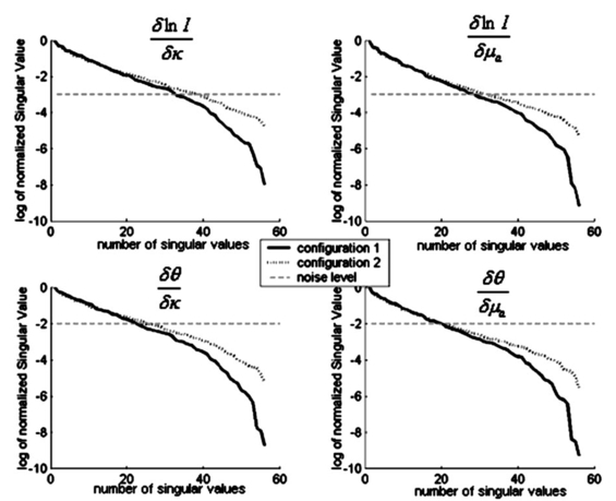

Taking noise level into consideration, Figure 4 and Table 2 show that more singular values exist above the practical noise threshold for each measurement type and optical property, if the preferential fiber arrangement (configuration 2) is used. The differences become more significant for higher signal-to-noise ratios. The increase at the noise level indicated in Figure 4 is about 2 to 8 singular values, which suggests that the data collected using this preferential fiber array configuration contains more information about the changes within the brain region. This in turn should correspond to more accurate image reconstruction, resulting in better resolution and quantitative localization.

Table 2

Number of singular values greater than the specified noise level for each measurement type and optical property for the homogeneous model, Figure 3(a).
	Configuration 1	Configuration 2	Increment
∂ ln ϕ/∂κ	32	38	+6
∂ ln ϕ/∂μ_a	28	31	+3
∂θ/∂κ	22	24	+2
∂θ/∂μ_a	20	19	−1

Given that the rat head is optically heterogeneous, it is important to investigate whether the heterogeneity will have any effect on those findings. Figure 5 and Table 3 show the singular values of each sensitivity map for each measurement type and optical property when a nonhomogeneous model is considered. Again taking noise into consideration, Figure 5 shows that more singular values (2 to 8 for the level indicated) exist above a given threshold for each measurement type and optical property, if the preferential fiber arrangement (configuration 2) is used. The differences are again more significant for higher signal-to-noise ratios.

Figure 5

Same as Figure 4 for the structured (heterogeneous) brain model.

Table 3

Number of singular values greater than the specified noise level for each measurement type and optical property for the structured model, Figure 3(b).
	Configuration 1	Configuration 2	Increment
∂ ln ϕ/∂κ	31	39	+8
∂ ln ϕ/∂μ_a	27	31	+4
∂θ/∂κ	20	23	+3
∂θ/∂μ_a	18	17	−1

3.2.

Image Reconstruction

Figure 6(a) (see Color Plate 2) shows the target μ_a image. Figure 6(b) presents the reconstructed image for equally spaced fibers when the model was assumed to have homogeneous optical properties while Figure 6(c) shows the corresponding image when the optical fibers are placed preferentially near the brain. The reconstructed images here and in the following section are those at the tenth iteration, and using a Celeron 600 Mhz Windows computer with 128 Mbyte RAM, computation time is about 10 s per iteration. Both arrangements yield a high-quality reconstruction of μ_a. The reconstructed central value in the absorbing inclusion is within a few percent of the true contrast in the region of interest. This result is very encouraging and confirms the initial findings from the singular value analysis, specifically that the preferential optical fiber arrangement should provide at least as much information about changes within the brain region as the conventional equally spaced fiber arrangement.

Figure 6

(a) The target μ_a image. Reconstructed images of absorption only, from noisy data calculated in the presence of an absorbing anomaly within the top region of the brain. (b) The homogeneous model where the data is from a single absorbing anomaly using fiber configuration 1. (c) The homogeneous model where the data is from a single absorbing anomaly using fiber configuration 2.

Given that the head is not optically homogeneous and that it contains structure, images have been reconstructed from data where background is heterogeneous and an absorption anomaly exists, again in the topside of the brain for both of the fiber arrangements. Figure 7 (see Color Plate 2) shows the model geometry plus the absorption reconstructions for both fiber arrangements. Overall, the recovered images are of comparable quality in terms of their visual characteristics. These results are significant, because they indicate that the preferential arrangement of optical fibers remains adequate in the presence of optical structure within the head.

Figure 7

Same as Figure 6. (a) The target μ_a image. (b) Reconstruction when the structured model and fiber configuration 1 are used. (c) Reconstruction when the structured model and fiber configuration 2 are used.

Quantitative comparisons of estimated and actual μ_a values along transects through the field of view for the homogeneous and structured model images in Figures 6 and 7 are shown in Figure 8. These plots indicate that the reconstructed μ_a values are very similar and quite accurate in the homogeneous case, whereas in the heterogeneous model they are less able to capture the degree of contrast within the localized absorbing inclusion. Interestingly, the preferentially spaced optical fiber configuration does a little better job of resolving the peak absorption in the inclusion, especially in the heterogeneous case, and may also exhibit modest improvements in edge resolution, but at the expense of increased levels of recovered property noise in the background.

Figure 8

Horizontal transects across the images of Figures 6 and 7, showing the absorption coefficient distribution for (a) the homogeneous background model and (b) the structured model. In both cases, the solid line shows the true absorption coefficient profile, the triangles show the reconstructed absorption distribution for fiber configuration 1, and the circles show the recovered absorption distribution for fiber configuration 2.

4. Discussion

This study focuses on evaluating two optical fiber configurations as possible arrangements for maximizing and improving the amount of information that can be extracted from the brain parenchyma through noninvasive NIR measurements on the rat cranium. An MRI image of the rat brain has been obtained and a 2-D finite element model of the head has been created. From this geometric model the sensitivity functions for the two different sets of optical fiber configurations have been calculated, one being an equally spaced arrangement around the head, and the other being preferentially arranged to the side nearest to the brain.

Singular value decomposition of these sensitivity maps within the brain was used to quantify and analyze the amount of information available from each optical fiber configuration. It was found that the preferential configuration of having the fibers grouped at the top of the head provided as much or more information from the brain region alone, relative to the evenly spaced fiber grouping. This was true whether the head model was assumed to be homogeneous or whether it was updated to contain optical property heterogeneity associated with the structure in the brain. In the case where the head is imaged using MRI and NIRS simultaneously, physical space limitations make it much easier to place fibers on one side of the cranium; hence, it is important from a practical standpoint to conclude that this fiber array configuration can be used without losing information about our region of interest.

Reconstructed images of the rat cranium from simulated data with noise where the presence of a localized change in absorption has been included confirm the general findings from the singular value analysis. Here, only images of absorption were reconstructed, assuming correct a priori scatter distribution, but the results (images) show that the preferential fiber arrangement set provides comparable image quality to a circumferential array with equally spaced fibers. Under homogenous conditions (except for the embedded inclusion), the μ_a reconstruction was quantitatively accurate, whereas image accuracy suffered when the background became optically heterogeneous. Also notable is an artificial effect that occurred in the heterogeneous reconstructed image, Figure 6(c); however, it would not cause much confusion since it is not near the region of our interest, the brain. Refinement of the reconstruction algorithm is an ongoing area of investigation, and the degree to which quantitative accuracy can be obtained in the heterogeneous case as well is the subject of a future study.

5. Conclusions

In a tomographic NIR imaging system, optical fibers arranged preferentially on one side of the rat head, near the brain, provide as much information, if not more, about optical changes within the brain as a fiber geometry that is uniformly distributed around the cross section of interest. This is particularly important in a practical setup where imaging of the rat head simultaneously using MRI and NIRS is highly constrained by the amount of space available. It has been shown that given accurate a priori information about structure and optical properties within the head, it is possible to computationally predict and image changes of absorption within the brain with excellent localization, using this preferential arrangement of fiber positions. The method discussed and employed in the study is also applicable to other studies, regardless of the organs of interest, reconstruction algorithm, or detection system.

Future work includes the development and use of more sophisticated algorithms, where structural information about the head is included in order to maximize the accuracy and spatial resolution of the optical properties within each region, as well as any changes within the brain. It is anticipated that the distribution of different chromophores can be correctly calculated and mapped within the brain with much finer spatial resolution and with more quantitative physiological significance than what is obtainable by using BOLD imaging alone. The experimental design and analysis for this work is presently under way.

Acknowledgments

This work has been sponsored by the National Institute of Health through grants NIH RO1 NS38471 and RO1 CA69544.

REFERENCES

1.

S. R. Arridge , P. van der Zee , M. Cope , and D. T. Delpy , “Reconstruction methods for infrared absorption imaging,” Proc. SPIE , 1431 204 –215 (1991). Google Scholar

2.

H. Jiang , K. D. Paulsen , U. L. Osterberg , B. W. Pogue , and M. S. Patterson , “Optical image reconstruction using frequency-domain data: simulations and experiments,” J. Opt. Soc. Am. A , 13 (2), 253 –266 (1996). Google Scholar

3.

S. R. Arridge , “Optical tomography in medical imaging,” Inverse Probl. , 15 (2), R41 –R93 (1999). Google Scholar

4.

B. W. Pogue , S. P. Poplack , T. O. McBride , W. A. Wells , K. S. Osterman , U. L. Osterberg , and K. D. Paulsen , “Quantitative hemoglobin tomography with diffuse near-infrared spectroscopy: pilot results in the breast,” Radiology , 218 (1), 261 –266 (2001). Google Scholar

5.

D. T. Delpy and M. Cope , “Quantification in tissue near-infrared spectroscopy,” Philos. Trans. R. Soc. London , 352 649 –659 (1997). Google Scholar

6.

B. Chance , Q. Luo , S. Nioka , D. C. Alsop , and J. A. Detre , “Optical investigations of physiology: a study of intrinsic and extrinsic biomedical contrast,” Philos. Trans. R. Soc. London , 352 707 –716 (1997). Google Scholar

7.

A. Kleinschmidt , H. Obrig , M. Requardt , K. D. Merboldt , U. Dirnagl , A. Villringer , and J. Frahm , “Simultaneous recording of cerebral blood oxygenation changes during human brain activation by magnetic resonance imaging and near-infrared spectroscopy,” J. Cereb. Blood Flow Metab. , 16 817 –826 (1996). Google Scholar

8.

A. Villringer and B. Chance , “Non-invasive optical spectroscopy and imaging of human brain function,” Trends Neurosci. , 20 (10), 435 –42 (1997). Google Scholar

9.

J. F. Dunn , Y. Zaim Wadghiri , B. Pogue , and I. Kida , “BOLD vs. NIR spectroscopy: will the best technique come forward?,” Adv. Exp. Med. Biol. , 454 103 –113 (1998). Google Scholar

10.

B. W. Pogue , T. O. McBride , C. Nwaigwe , U. L. Osterberg , J. F. Dunn , and K. D. Paulsen , “Near-infrared diffuse tomography with apriori MRI structural information: testing a hybrid image reconstruction methodology with functional imaging of the rat cranium,” Proc. SPIE , 3597 484 –492 (1999). Google Scholar

11.

B. W. Pogue and K. D. Paulsen , “High resolution near infrared tomographic imaging simulations of rat cranium using apriori MRI structural information,” Opt. Lett. , 23 (21), 1716 –1718 (1998). Google Scholar

12.

V. Ntziachristos , A. G. Yodh , M. Schnall , and B. Chance , “Concurrent MRI and diffuse optical tomography of breast after indocyanine green enhancement,” Proc. Natl. Acad. Sci. U.S.A. , 97 (6), 2767 –2772 (2000). Google Scholar

13.

J. Chang , H. L. Graber , P. C. Koo , R. Aronson , S. S. Barbour , and R. L. Barbour , “Optical imaging of anatomical maps derived from magnetic resonance images using time independent optical sources,” IEEE Trans. Med. Imaging , 16 68 –77 (1997). Google Scholar

14.

J. P. Culver , V. Ntziachristos , M. J. Holboke , and A. G. Yodh , “Optimization of optode arrangements for diffuse optical tomography: a singular-value analysis,” Opt. Lett. , 26 (10), 701 –703 (2001). Google Scholar

15.

M. Schweiger , S. R. Arridge , M. Hiraoka , and D. T. Delpy , “The finite element model for the propagation of light in scattering media: boundary and source conditions,” Med. Phys. , 22 1779 –1792 (1995). Google Scholar

16.

S. R. Arridge and M. Schweiger , “Photon-measurement density functions. Part 2: Finite-element-method calculations,” Appl. Opt. , 34 8026 –8037 (1995). Google Scholar

17.

T. O. Mcbride, “Spectroscopic reconstructed near infrared tomographic imaging for breast cancer diagnosis,” PhD Thesis, Dartmouth College, NH (2001).

18.

M. Schweiger and S. R. Arridge , “Optical tomographic reconstruction in a complex head model using a priori region boundary information,” Phys. Med. Biol. , 44 2703 –2722 (1999). Google Scholar

19.

M. Cope , P. Van der zee , M. Essenpreis , S. R. Arridge , and D. T. Delpy , “Data analysis methods for near infrared spectroscopy of tissue: problems in determining the relative cytochrome aa₃ concentration,” Proc. SPIE , 1431 251 –262 (1991). Google Scholar

20.

M. Firbank , M. Hiraoka , M. Essenpreis , and D. T. Delpy , “Measurement of the optical properties of the skull in the wavelength range 650-95-nm,” Phys. Med. Biol. , 38 503 –510 (1993). Google Scholar

21.

C. R. Simpson , M. Kohl , M. Essenpreis , and M. Cope , “Near infrared optical properties of ex-vivo human skin and subcutaneous tissues measured using the Monte Carlo inversion technique,” Phys. Med. Biol. , 43 2465 –2478 (1998). Google Scholar

22.

C. R. Simpson , M. Kohl , M. Essenpreis , and M. Cope , “Near Infrared optical properties of ex-vivo human skin and sub-cutaneous tissues measured using the Monte Carlo inversion technique,” Phys. Med. Biol., 43 (9), 2465 –2478 (1998). Google Scholar

Citation Download Citation

Heng Xu, Hamid Dehghani, Brian W. Pogue, Roger Springett, Keith D. Paulsen, and Jeff F. Dunn "Near-infrared imaging in the small animal brain: optimization of fiber positions," Journal of Biomedical Optics 8(1), (1 January 2003). https://doi.org/10.1117/1.1528597

Published: 1 January 2003

Access the abstract

JOURNAL ARTICLE
9 PAGES

DOWNLOAD PAPER SAVE TO MY LIBRARY

GET CITATION

CITATIONS

Cited by 87 scholarly publications and 1 patent.

Explore citations on Lens.org

RIGHTS & PERMISSIONS

Get copyright permission Get copyright permission on Copyright Marketplace

KEYWORDS

Brain

Optical properties

Head

Optical fibers

Neuroimaging

Data modeling

Absorption

1.

Introduction