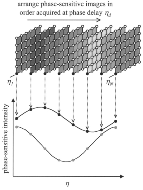
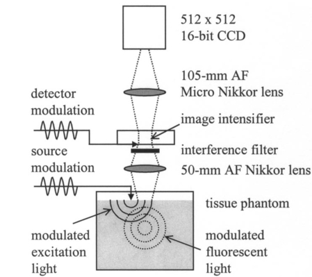
1.

Introduction

Since 10 of breast cancers are not detected by x-ray mammography,¹ researchers have initiated efforts to develop complementary or alternative screening technologies to increase the overall sensitivity and specificity of detection. Near-IR (NIR) imaging with light at wavelengths ranging between 700 and 900 nm has recently emerged as a potential diagnostic tool. At these wavelengths, photons are multiply scattered and minimally absorbed by tissues. Hawrysz and Sevick-Muraca² recently reviewed several NIR imaging techniques directed toward breast cancer detection. To detect and delineate the disease (1) light must be differentially absorbed and/or scattered by normal and diseased tissues; (2) photons, whose different times of flight suggest spatial variability in the optical absorption and/or optical scattering properties of tissues, must be rapidly, precisely, and accurately discriminated by a detector; and (3) a 3-D map of optical properties must be iteratively updated by a robust and computationally efficient inversion algorithm until experimental measurements of multiply scattered light approximate those predicted by an appropriate mathematical model of light propagation in tissue.

Using frequency-domain photon migration (FDPM) techniques, investigators^{3 4 5} have successfully constructed optical mammograms that delineate breast cancer based on a disparity in blood volume, which affects optical absorption differences between normal and diseased tissues. FDPM refers to the propagation of intensity-modulated NIR light through a multiply scattering medium. The intensity-modulated light originates from a source whose intensity is sinusoidally modulated, typically at a radio frequency. The detected light, whose intensity is modulated at the same frequency, is phase shifted and amplitude attenuated relative to the source light. FDPM measurements of phase and modulation amplitude are indicative of photon times of flight and ultimately the spatial distribution of tissue optical properties that govern the propagation of intensity-modulated light. As revealed by FDPM measurements, a disparity in blood volume between normal and diseased tissues is absent for early tumors smaller than a few millimeters in size.⁶ Thus, current state-of-the-art FDPM techniques in NIR optical mammography are designed for detection of late-stage disease.

Early detection of breast cancer reduces its mortality.⁷ To facilitate early detection and to enable the detection of metastatic disease, fluorescent agents that excite and re-emit in the NIR can be introduced to enhance tissue contrast.⁸ Accordingly, the inversion algorithm is amended for incorporation of fluorescence emission data and a model for fluorescent light propagation to isolate and characterize disease from parameters that mediate enhanced tissue contrast. Contrast could result from an agent that extravasates through the tumor hyperpermeable neovasculature and either pools in the extracellular space^{9 10 11 12} or selectively target tumor cells.^{11 12 13 14 15 16 17} Contrast could also result from an alteration in fluorescence quantum efficiency¹⁸ or fluorescence lifetime¹⁹ upon partitioning of an agent into diseased tissues. These parameters significantly impact measurements of fluorescence FDPM. Fluorescence FDPM refers to the propagation of intensity-modulated NIR fluorescent light that originates from tissue-laden fluorophores, which are excited by propagated intensity-modulated NIR light that originates from a source located on the tissue surface. Fluorescence FDPM measurements are further phase delayed and amplitude attenuated, which suggests the possibility of improved contrast between normal and diseased tissues.^{20 21}

Reported here are the measurement precision and accuracy representative of an intensified charge-coupled device (ICCD) homodyne detection system, adapted from systems described in the literature^{22 23} for the acquisition of fluorescence FDPM measurements. While these and other similar systems have been employed for fluorescence lifetime imaging microscopy^{22 24 25 26 27} (FLIM) and, on a more limited basis for FDPM (Refs. 23 and 28), reports detailing the precision and accuracy of FDPM measurements of phase and modulation amplitude have not been published. Measurement precision and accuracy crucially impact the solution to the underdetermined inverse problem, where the number of unknowns largely exceeds the number of knowns. Researchers active in the area of FLIM have reported only the accuracy of recovered fluorescence lifetimes. Described in the following sections are the ICCD homodyne detection system and the materials and methods employed to assess its measurement precision and accuracy for a data acquisition time that is clinically feasible. The results gathered from this investigation are then presented and compared to those obtained with single-pixel heterodyne detection systems also located in the laboratory.

2.

Materials and Methods: ICCD Homodyne Detection System

2.1.

Instrumentation

Figure 1 presents the ICCD homodyne detection system, which is also described by Reynolds et al.;²⁹ The detection system consists of three major components, which include (1) a CCD camera (Photometrics Ltd., series AT200, model SI512B, Tucson, Arizona), which houses a 512×512 array of photosensitive detectors and an output amplifier that converts analog data to 16-bit digital data at a rate of 40,000 pixels/s; (2) a gain-modulated image intensifier (ITT Industries Night Vision, model FS9910C, Roanoke, Virginia), which is used to facilitate measurements of FDPM; and (3) oscillators, which are used to sinusoidally modulate the intensity of a laser diode light source and the intensifier gain at the same frequency (homodyne mixing). A 1-V, 100-MHz sinusoidal signal, which is added to the dc bias voltage of the laser diode, is provided by the first oscillator (Marconi Instruments Ltd., model 2022D, Hertfordshire, England). Provided by a second oscillator (Programmed Test Sources, Inc., model 310, Littleton, Massachusetts), a 1-V, 100-MHz sinusoidal signal is amplified to 22 V (provided by ENI Technology, Inc., model 604L, Rochester, New York) and added to the dc bias voltage of the intensifier photocathode (provided by GBS Micro Power Supply, model PS20060500, San Jose, California). The oscillators are phase-locked by a 10-MHz reference signal. A phase-sensitive,²² steady-state image is produced on the intensifier phosphor screen as a result of homodyne frequency mixing. The phase-sensitive, steady-state image is optically relayed to the CCD array using a 105-mm AF Micro Nikkor lens (Nikon Corp., Tokyo, Japan).

Figure 1

Experimental setup used to assess FDPM measurement precision.

2.2.

Data Acquisition

As detailed by Reynolds et al.;,²⁹ FDPM data are gathered using a computer program (PMIS Image Processing Software, Photometrics Ltd., Tucson, Arizona) that directs the following procedure. Via an IEEE-488 general purpose interface bus (GPIB) (National Instruments Corp., Austin, Texas), the phase of the intensifier modulation is evenly stepped, or delayed, N times between 0 and 360 deg relative to the phase of the laser diode modulation. At each phase delay η_d, a phase-sensitive image is acquired by the CCD camera for a given exposure time. The 512×512 array of CCD pixels is “binned” down to a 128×128 array during charge readout and before signal digitization. Binning, or the addition of electronic charge in adjacent pixels, reduces the resolution of a CCD array, accelerates data acquisition, and improves the signal-to-noise ratio³⁰ (SNR). Following completion of the 360 deg loop, the laser diode is inactivated, and a steady-state image is acquired by the CCD camera using the same exposure time. This image contains ambient light, dark current, and read noise. Dark current refers to thermally generated charge, while read noise is introduced at the output amplifier.³⁰ Directed by a Matlab routine (The Mathworks, Inc., Natick, Massachusetts), (1) the steady-state image is subtracted from the phase-sensitive images; (2) the corrected phase-sensitive images are arranged in the order that they were acquired (see Figure 2); and (3) a fast Fourier transform (FFT) is performed at each pixel (i,j) to calculate phase, θ, and modulation amplitude, I _ac , using the following relationships:²⁹

Eq. (1)

$$\theta (i,\mathit{j})=\text{arctan}\left(\frac{\text{IMAG}[\mathit{I}{({\mathit{f}}_{\text{max}})}_{ij}]}{\text{REAL}[\mathit{I}{({\mathit{f}}_{\text{max}})}_{ij}]}\right),$$

Eq. (2)

$${\mathit{I}}_{\text{ac}}(\mathit{i},\mathit{j})=\frac{[{\{\text{IMAG}[\mathit{I}{\left({\mathit{f}}_{\text{max}}\right)}_{ij}]\}}^2+\{\text{REAL}{{[{\mathit{I}\left({\mathit{f}}_{\text{max}}\right)}_{ij}]\}}^2]}^{1/2}}{N/2},$$

where I(f ) is the Fourier transform of the phase-sensitive intensity data I(η_d); IMAG[I(f _max )] and REAL[I(f _max )] are the imaginary and real components in the digital frequency spectrum that best describe the sinusoidal data. I _dc (i,j), the average intensity at each pixel, is also calculated.

Figure 2

ICCD homodyne data acquisition.

3.

Materials and Methods: Assessment of Measurement Precision

3.2.

Data Acquisition Parameters and Quantities Indicative of Measurement Precision

Measurement precision relied on the selection of three data acquisition parameters, which included (1) the number of phase delays, N (8, 16, or 32), introduced between the oscillators used to modulate the laser light intensity and intensifier gain; (2) the number of frames or phase-sensitive images collected by the ICCD per phase delay; and (3) CCD exposure time (0.2, 0.4, or 0.8 s) for each frame. Data acquisition parameters were chosen such that the data acquisition time, equivalent to the product of phase delays, exposure time, and frames and excluding the time necessary to readout and digitize charge, totaled 2 min, which is reasonable for future application of the ICCD technology in the clinical setting. The 2ⁿ data points are most efficiently managed²⁹ by the Matlab FFT, which supported the reported sampling of phase delays. Also, no more than 64 phase delays can be used. Interpreted by the PTS 310 oscillator, ASCII codes for N⩽64 are only available. Previous clinical work with large canines^{9 11} warranted the reported sampling of exposure times, which were necessary for sufficient detection of fluorescence generated in vivo.

Figure 3 depicts the data analysis procedure employed to assess measurement precision. After compiling a number of θ, I _ac , and I _dc images equal to the number of frames (up to 75) acquired per phase delay, images of θ error (□), I _ac error (■), and mean I _dc () were computed. For each pixel, θ error or precision refers to the standard deviation (STD) in phase, and I _ac error or precision refers to the STD in I _ac divided by its mean. Data were acquired for four different normalized irradiances and pooled together.

Figure 3

Data analysis procedure used to assess FDPM measurement precision; □ obtained from FFT of phase-sensitive images, (dotted box) obtained from mean of phase-sensitive images, ■ obtained from STD of θ images, ▪ obtained from STD/mean of I _ac images, and  obtained from mean of I _dc images.

4.

Materials and Methods: Assessment of Measurement Accuracy

4.2.

Experimental Setup

Figure 4 presents the experimental setup employed to assess FDPM measurement accuracy. Produced by a 25-mW laser diode (Thorlabs, Inc., model HL7851G, Newton, New Jersey), 784-nm excitation light, whose intensity was sinusoidally modulated at 100 MHz, was delivered via fiber optic [1000-μm core diameter, 0.39 numerical aperture (NA), Thorlabs, Inc., model FT-1.0-EMT, Newton, New Jersey] to a tissue phantom, 22 cm in diameter and 12 cm in height. The output of the fiber optic was positioned flush with the surface of a tissue-like solution contained within the phantom. The optical power and wavelength of the laser light were maintained with a laser diode driver (Melles Griot, model 06DLD203, Boulder, Colorado). The phantom contained 4.5 l of 1 Liposyn, a fat emulsion whose scattering properties mimic those of tissue. The 1 solution was prepared by volumetric dilution of 20 stock solution (Abbott Lab., North Chicago, Illinois) with deionized, ultrafiltered water. Indocyanine green (Sigma-Aldrich Co., St. Louis, Missouri), a fluorescent contrast agent approved by the Food and Drug Administration (FDA) for diagnostic purposes, was initially dissolved in deionized, ultrafiltered water and then added to the 4.5 l of 1 Liposyn to formulate a 0.1-μM solution. An 830-nm bandpass interference filter (10 nm FWHM, CVI Laser Corp., model F10-830.0-4, Albuquerque, New Mexico) was placed before the image intensifier to isolate 830-nm fluorescent light emanating from a 3.1×3.1 cm ² area on the solution surface.

Figure 4

Experimental setup used to assess FDPM measurement accuracy.

5.

Results and Discussion: Measurement Precision

Figure 5 shows how precisely I _ac and θ are measured using the ICCD homodyne detection system for 8, 16, and 32 phase delays introduced between the oscillators used to modulate the laser light intensity and intensifier gain at 100 MHz. A 0.2-s exposure time was used to collect the phase-sensitive intensities per phase delay. The trends observed in Figure 5 are similar to those, which are not shown, obtained for the use of 0.4- and 0.8-s exposure times. Table 1 lists the mean I _ac error and mean θ error as a function of phase delays and exposure time. Mean I _ac error and mean θ error are minimized at ±0.46 and ±0.26 deg, respectively, which correspond to the use of 32 phase delays and a 0.8-s exposure time. Figure 5 indicates that I _ac error and θ error diminish in response to elevated mean I _dc . Since SNR improves with increased I _dc these results are expected. A comparison of Figures 6(a) and 6(c), which plot phase-sensitive intensity versus 32 phase delays for 2 pixels in the detection area, confirms that FDPM measurement precision improves when mean I _dc increases. A comparison of Figures 6(b) and 6(d), which plot phase-sensitive intensity versus 8 phase delays for the same two pixels, provides further confirmation. Figure 5 also reveals that I _ac error and θ error diminish as a greater number of phase delays are used. When noise significantly impacts a measurement, use of a greater number of points (or phase delays) to construct a sine wave results in a more reliable computation of I _ac , I _dc , and θ. A comparison of Figures 6(c) and 6(d) best illustrates this improvement in measurement precision. As noted in Table 1, mean errors in measurements acquired using the 0.2- and 0.4-s exposure times are similar, which is expected because the means of mean I _dc data acquired using these exposure times are similar. Mean errors in measurements acquired using the 0.8-s exposure time are smaller than those obtained using the 0.2- and 0.4-s exposure times because the means of mean I _dc data acquired using the 0.8-s exposure time exceed the means of mean I _dc data acquired using the 0.2- and 0.4-s exposure times. CCD charge storage capacity was best sampled for the trials corresponding to the use of the 0.8-s exposure time.

Figure 5

Data acquired using the ICCD homodyne detection system illustrating precision in measurement of I _ac and θ; I _ac error, or STD (I _ac )/mean(I _ac ), is reported for the use of (a) 8, (b) 16, and (c) 32 phase delays; θ error, or STD(θ), is also reported for the use of (d) 8, (e) 16, and (f) 32 phase delays. A 0.2-s exposure time was used to collect the phase-sensitive intensities per phase delay. Data corresponding to normalized irradiances of 2.1×10⁻², 3.5×10⁻², 5.8×10⁻², and 1.5×10⁻¹ were pooled together.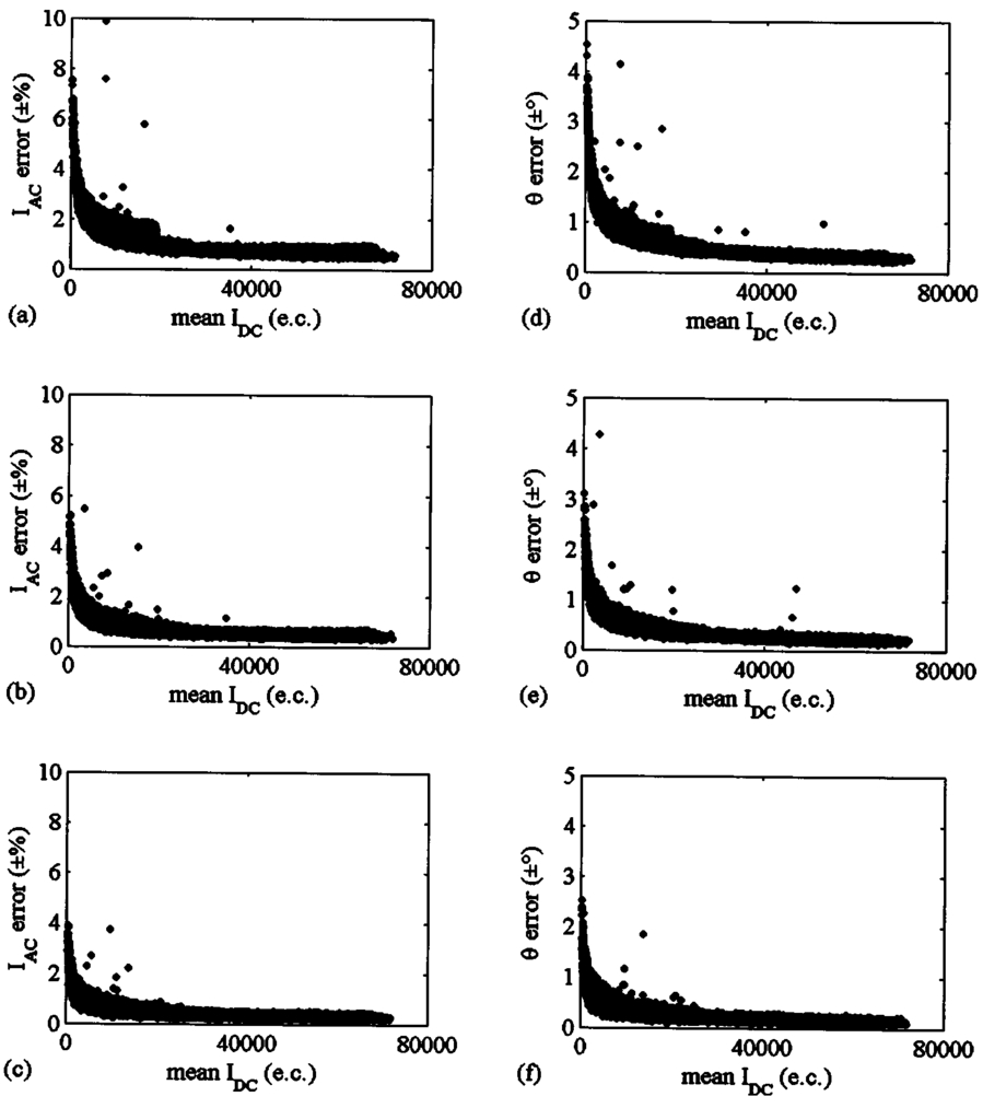

Figure 6

Data depicting precision of homodyne measurement for two CCD pixels exposed for 0.2 s. High mean I _dc can be observed for the acquisition of (a) 19 sine waves, each containing 32 data points (for the use of 32 phase delays), and (b) 75 sine waves, each containing 8 data points (for the use of 8 phase delays). Low mean I _dc can be observed for the acquisition (c) 19 sine waves, each containing 32 data points, and (d) 75 sine waves, each containing 8 data points.

Table 1

To identify the principal source of noise that corrupts the phase-sensitive intensity measurements, I _dc SNR are plotted versus mean I _dc for the use of 8, 16, and 32 phase delays in Figure 7. A 0.2-s exposure time was used to collect the phase-sensitive intensities per phase delay. Similar results, which are not shown, were obtained for the use of 0.4- and 0.8-s exposure times. Figures 7(a) through 7(c) appear to indicate a linear relationship between I _dc SNR and mean I _dc . To confirm this observation, mean I _dc data and corresponding I _dc SNR data are collected in bins and averaged, and the results of this procedure are presented in Figures 7(d) through 7(e). The “length” of each bin along the abscissa axis is 200 e.c. In other words, the abscissa of any data point in Figures 7(d) through 7(e) represents the average of mean I _dc data collected in a bin for which [max(mean I _dc )–min(mean I _dc )⩽200 e.c.], and the ordinate represents the average of I _dc SNR data corresponding to the mean I _dc data collected in the bin. Each data point in Figures 7(a) through 7(c) belongs to only one bin in Figures 7(d) through 7(e). Figures 7(d) through 7(e) indeed confirm a linear relationship between I _dc SNR and mean I _dc . For comparison, solid lines, which represent the square root of the binned mean I _dc data, are plotted in these same figures. SNR is proportional to the square root of the signal for photon-noise-limited operation.³⁵ Given that the data in Figures 7(d) through 7(e) are plotted on a log-log scale, this proportionality would be observed as a constant offset in the ordinate direction between the predicted (solid line) and measured data (points). Since this constant offset is indeed observed, operation of the ICCD homodyne detection is photon noise limited for the experimental conditions used to gather the data presented in Figures 5 through 7.

Figure 7

Data illustrating relationship between I _dc SNR and mean I _dc for the use of (a) 8, (b) 16, and (c) 32 phase delays. A 0.2-s exposure time was used to collect the phase-sensitive intensities per phase delay. Data corresponding to normalized irradiances of 2.1×10⁻², 3.5×10⁻², 5.8×10⁻², and 1.5×10⁻¹ were pooled together. To better illustrate the relationship between I _dc SNR and mean I _dc , data corresponding to the use of (d) 8, (e) 16, and (f) 32 phase delays are collected in bins and averaged. The solid lines represent the square root of the binned mean I _dc data.

Other investigators in the laboratory have reported the acquisition of single-pixel heterodyne measurements of I _ac and θ with a mean precision of ±0.090 and ±0.041 deg, respectively,³⁶ which reflects better measurement reproducibility when compared to that obtained with the multipixel ICCD homodyne detection system. Unlike homodyne frequency mixing, heterodyne frequency mixing involves modulating the source light intensity and detector gain at slightly different frequencies. The frequency difference, or cross-correlation frequency, is of the order of hertz. The cross-correlated signal retains the phase and modulation amplitude characteristics of the high-frequency signal entering the detector. The single-pixel experimental setup incorporated a pair of fiber optics that transmitted source and detected signals to and from a multiply scattering medium, respectively. Measurements were acquired at modulation frequencies spanning 10 to 100 MHz and source-detector separation distances spanning 0.7 to 1.5 cm. A 100-Hz cross-correlated signal was sampled for 6 s to yield 2048 values of I _ac and θ at each modulation frequency and source-detector separation distance. Note that I _ac and θ were computed from an FFT of 30 data points acquired per approximately three-tenths of a sinusoidal cycle. Therefore, on a per pixel basis, a much greater amount of data is collected by the single-pixel detection system for a given position and period of time when compared to the capabilities of the multipixel detection system, which serves as an area detector. Although it is incorrect to directly compare the measurement precision characteristics of these two detection systems given differences in light input and detector type (photomultiplier tube versus ICCD), the results are reported nonetheless to illustrate their measurement capabilities. Furthermore, the authors recognize that the range of values present in the FDPM images impacts ICCD homodyne measurement precision. Smaller ranges would result in improved precision and vice versa for larger ranges. It is important to note that a dynamic range of 2¹⁶ is used to report a range of values present in one CCD image. On the other hand, a dynamic range at least five orders of magnitude in size is used to report a measurement acquired at a single point with the photomultiplier tube. Therefore, the performance of a single-pixel heterodyne detection system in terms of measurement precision is expected to surpass that of an ICCD homodyne detection system.

Timing considerations prevent operating the ICCD detection system in heterodyne mode for acquisition of FDPM measurements. One hundred data points obtained by the single-pixel heterodyne detection system are employed in the construction of one sinusoidal cycle, which corresponds to a data acquisition rate of 10 kHz for a cross-correlation frequency of 100 Hz. The maximum rate at which an image with a resolution of 128×128 pixels is acquired by the ICCD detection system is approximately 3 Hz, given that the time required to digitize all charge, which is approximately 0.4 s, greatly exceeds the time required to integrate charge. Supported by previous clinical work with large canines,^{9 11} integration times of 0.2 s or greater are needed to sufficiently detect fluorescent signals generated in vivo. Therefore, a reasonable maximum rate at which a fluorescence image can be acquired by the ICCD detection system is approximately 2 Hz. (These estimates of imaging rate neglect the time associated with clearing the CCD of excess charge prior to integration, delays in opening and closing the shutter, and shifting charge out of the CCD to the output amplifier.) The minimum cross-correlation frequency that can be provided by the sophisticated instrumentation available in the laboratory is 1 Hz. Therefore, at best, only 2 data points can be acquired per sinusoidal cycle for each pixel in the multipixel detection system when implementing a heterodyne detection scheme. This limited amount of information is inadequate for precisely and accurately determining phase and modulation amplitude.

French et al.;²⁸ describe an ICCD heterodyne detection system that has been employed to obtain FDPM measurements. Their intensifier gain is modulated at 100 MHz (the frequency at which the intensity of the laser light source is sinusoidally varied) plus a cross-correlation frequency of 15 Hz. The camera has an 8-bit analog-to-digital (A/D) converter, which drastically improves the imaging rate. Given an imaging rate of 60 Hz, they are able to obtain 4 data points per sinusoidal cycle. The authors have failed to report measurement precision, which prevents a direct comparison of their system and the ICCD homodyne detection system presented in this paper.

6.

Results and Discussion: Measurement Accuracy

Figure 8 compares experimental (points) and predicted (line) measurements of fluorescence I _ac and θ acquired at distances ranging between 0.71 and 3.6 cm from the incident excitation point source. Measurements of I _ac and θ exhibit a mean accuracy of 17 and 1.9 deg, respectively. Greatest measurement accuracy was obtained at locations closest to the point source. Generally, measurement error increases with increasing distance from the point source, which most likely results from deteriorating measurement precision associated with an exponential decrease in I _ac I _dc , and hence SNR. Other explanations for observed discrepancies between experiment and theory include (1) a failure to accurately quantitate optical and fluorescent properties characteristic of the tissue phantom, (2) the inability to accurately position the fiber optic with respect to the CCD detection area and the surface of the tissue-like medium, and (3) an inherent limitation to the analytical solution. When deriving the analytical solution, Li et al.;³¹ neglected to comply with a restriction imposed by use of the extrapolated zero fluence boundary, which necessitates an absence of fluorophores within the space located between the physical and image tissue boundaries. Nevertheless, after comparing the analytical solution to results generated by a finite difference algorithm, they observed better than 3 accuracy in I _ac and 1.2 deg accuracy in θ for a source-detector separation distance of 2 cm and modulation frequencies spanning 0 to 800 MHz.

Figure 8

Data acquired using the ICCD homodyne detection system depicting accuracy in measurement of fluorescence I _ac and θ. Normalized and referenced measurements (gray circles) of (a) I _ac and (b) θ are compared to theoretical predictions (solid line), which enables calculation of (c) relative error for I _ac and (d) absolute error for θ. Thirty-two phase delays and a 0.4-s exposure time were employed to acquire the data.

In a previous study conducted in the laboratory using a single-pixel heterodyne detection system,³⁷ measurements of fluorescence I _ac and θ exhibited a mean accuracy of 23 and 4.9 deg, respectively, when compared to 3-D finite difference predictions for source-detector separation distances spanning 1.0 to 4.2 cm and a modulation frequency of 100 MHz. Discretization error associated with finite differencing and low SNR at large source-detector separation distances may have led to these large measurement errors. These results suggest that actual experimental single-pixel and multipixel detection systems comparably monitor fluorescence FDPM. Although differences in light input and detector type again preclude a proper comparison of the detection systems, the results are reported nonetheless to illustrate their measurement capabilities.

7.

Summary

This paper presented the precision and accuracy of FDPM measurements acquired using an ICCD homodyne detection system, developed to augment the quantity of data acquired within clinically relevant imaging times. Constrained by a data acquisition time of two minutes, mean precision was maximized at ±0.46 and ±0.26 deg for ICCD measurements of modulation amplitude and phase, respectively. Measurement accuracy was assessed by comparing experimental fluorescence measurements, acquired from the surface of a homogeneous medium illuminated with an intensity-modulated point source of light, to predicted values computed from an analytical solution to the coupled photon diffusion equations. ICCD measurement accuracy relies on model assumptions, independent tissue property measurements, and signal levels. Nonetheless, mean accuracy, which was 17 and 1.9 deg for measurements of I _ac and θ, respectively, is comparable to that obtained with a single-pixel heterodyne detection system, which has been used to create 3-D maps of tissue optical properties characteristic of heterogeneous tissue-like media.^{38 39} These results suggest that like single-pixel measurements, fast ICCD measurements of fluorescence FDPM may be sufficiently accurate and precise for incorporation into an Bayesian inversion algorithm^{40 41} that accounts for measurement error during the recovery of tissue optical and fluorescent properties.