2.1.

Optical Property Sets

The first task in this study was to generate radial reflectance distributions for a large number of optical property (μ_a,μ_s ^′) combinations. Two lists, each containing 30 optical property pairs, were developed: a “uniform” list including μ_a values of 1, 5, 10, 15, 20, and 25 cm ⁻¹ and μ_s ^′ values of 5, 10, 15, 20, and 25 cm ⁻¹ ; as well as a “random” list generated using a uniform random distribution over a μ_a range of 1 to 25 cm ⁻¹ and a μ_s ^′ range of 5 to 25 cm ⁻¹ . One simulated and one experimentally determined radial distribution were generated for each optical property pair. The resulting 120 distributions were divided into four datasets labeled by how the optical property pair and the radial distribution were developed (simulated uniform, simulated random, measured uniform, or measured random).

2.2.

Simulation of Reflectance Data

A weighted photon Monte Carlo model of light transport was developed to calculate radial reflectance distributions for given optical property pairs (μ_a,μ_s ^′). ^{3 4} A brief overview of the Monte Carlo method is provided here, while excellent detailed coverage is available elsewhere.^{20 21} This technique involves the repeated generation of random numbers and calculation of stochastic relations to simulate the random walk of a large number of individual photons as they propagate through tissue. These relations are used to calculate parameters such as the angle and location of photon launch, the step size between scattering events, the angle of scatter, refraction/reflection at surfaces, and photon termination. Photons were launched in a uniform distribution over all positions on a circle representing the fiber face, as well as in a uniform distribution over all angles within the cone specified by NA=n_i sinθ, where NA is the numerical aperture, n_i is the index of refraction of the tissue, and θ is the exit angle (measured from the normal to the tissue surface). To replicate the conditions of the tissue phantom measurements, simulations incorporated a fiber NA of 0.22 and a fiber index of refraction of 1.45. It should also be noted that the index of refraction of water (n_i=1.37) was used both because of the high water content of the Intralipid solutions and to approximate the index of refraction of liver tissue.²² For all simulations, the μ_s value used in Monte Carlo algorithms was calculated from μ_s ^′ and a g of 0.9. This value of g is within the range that is relevant for tissue. Photons exiting the tissue at the surface were subjected to a similar angular restriction prior to detection. The location of “detected” photons were recorded in radial bins 0.025 mm in width.

2.3.

Tissue Phantoms Measurements

Diagrams of the experimental setup and fiber optic probe used to perform diffuse reflectance measurements are presented in Fig. 1. For all tissue phantom measurements, the source was a temperature-controlled, 675-nm laser diode (Edmund Industrial Optics, Barrington, New Jersey) with a power level of 5 mW. This source was used due to its low cost, stability, and ease of comparison with prior studies. For the phantom measurements, actual wavelength is much less important than the optical property range, which was made to correspond to biological tissues in the UVA to VIS range. The input power was adjusted with neutral density filters. A custom-designed fiber optic probe (FiberTech Optica, Ontario, Canada) was used to deliver light from the source to the sample and guide diffuse reflectance from the sample to the detector. All fibers had a core diameter of 0.2 mm and an NA of 0.22. The source leg of the probe consisted of a single fiber, while the detection leg consisted of six fibers spaced at center-to-center distances of 0.23, 0.67, 1.12, 1.57, 2.01, and 2.46 mm from the source fiber (labeled n=1 to n=6). The remaining area of the probe face was blackened to minimize reflections. The probe was submersed in liquid phantom material contained in a cuvette that was large enough to provide a semi-infinite medium—no change in reflectance was produced when larger cuvette sizes were used. The detection leg terminated at an inverted microscope (Diavert, Leitz, Germany) with the output imaged onto a CCD camera (Model CH250, Photometrics, Tuscon, Arizona). Images were acquired and stored on a personal computer. The linearity of the CCD images was verified using a power meter (Labmaster, Coherent, Incorporated, Santa Clara, California).

Figure 1

Diagram of (a) experimental setup and (b) fiber optic probe face. Illumination and collection fibers on probe face are represented by shaded and nonshaded circles, respectively.

Tissue phantoms were generated for each of the 60 optical property pairs on the uniform and random lists. These phantoms were created by combining varying concentrations of a scatterer (Intralipid®, Baxter Healthcare Corporation, Deerfield, Illinois), an absorber (N-4754, Water Soluble Nigrosin, Sigma Chemical Company, Saint Louis, Missouri), and distilled water. Absorption coefficients were determined based on a μ_a of 34 cm ⁻¹ for a stock nigrosin solution at 675 nm, as determined from transmission measurements. Scattering coefficients were determined through linear scaling given a μ_s ^′ of 18 cm ⁻¹ at 675 nm for a 15 concentration of the stock 10 Intralipid, as calculated from spectrophotometer measurements and the inverse adding doubling technique,²³ assuming that g=0.72. ²⁴

It should be noted that while g=0.72 represents a highly forward-scattering medium, it is outside the range of g values (g⩾0.9) indicated by Graff et al.;¹ for validity with the similarity relation. In a prior study, Kienle et al.;⁴ evaluated the validity of invoking the similarity relation¹ for Liposyn samples for which a g of 0.8 was measured by performing Monte Carlo calculations using different g values but the same μ_s ^′. In this prior study, the maximum difference in reflectance between the g=0.8 case and g=0.95 cases was found to be 8. We performed results that indicated excellent agreement between reflectance distributions calculated for g=0.9 and 0.72 over most of the optical property range and for all fibers. These results are consistent with a prior study that analyzed distributions for values of g from 0.7 to 0.99.⁹

2.4.

Development of Inverse Models

Raw reflectance data from computational or experimental results were preprocessed as follows:

The method of PLS has been reviewed previously.^{11 12} This approach involves the determination of a calibration matrix B, by regression between the two matrices X and Y that represent the reflectance and corresponding optical property matrices, respectively. The matrix X contains m=5 columns of reflectance data (representing five fiber locations). The matrix Y contains p=2 columns (the two optical properties that characterize each sample). The PLS algorithm employs a singular value decomposition function to iteratively decompose the optical property and reflectance data and form a model matrix B:

The NN algorithm involved a feed-forward backpropagation network based on a Levenburg-Marquardt training function.^{26 27} The input layer had five nodes, corresponding to the five nonzero S values, and the output layer contained two nodes, one for each of the two optical properties predicted. A hyperbolic tangent sigmoid transfer function was used in the hidden layer and a linear transfer function in the outer layer. Training of the network necessitated dividing the calibration data into three subsets. Approximately half of the calibration data was used for the training set, a quarter for the validation set, and a quarter for the testing set. The algorithm employed a validation set to terminate training early if the model performance failed to improve over several iterations, and used a testing set to verify that the network was generalizing well. Typically, algorithm training was terminated when improvements in model performance slowed to a minimal level.

2.5.

Measurements of Ex Vivo Tissue

Further evaluation of our approach to optical property determination was performed using ex vivo biological tissue samples. Bovine liver samples were interrogated due to their relative homogeneity and evidence that their optical properties would be within the range of interest.^{28 29} Measurements were performed on fresh tissue purchased from a local market and were approximately 48-h post mortem at the time of use. The tissue was refrigerated and wrapped in plastic to minimize water and blood loss. The experimental setup was identical to that shown in Fig. 1, with the exception that two different sources were used: helium neon lasers at wavelengths of 543 and 633 nm (Models 1508 and 1653, JDS Uniphase, San Jose, California). Laser power delivered to the tissue was 0.3 mW at 543 nm and 0.05 mW at 633 nm. For each wavelength, two measurements were taken at each of three different locations. Reflectance data were processed as described previously. For each measurement, the distribution S was then used as input to the NN model developed from simulated reflectance data with uniform optical properties (Table 1, cases 1 to 4). Optical property estimations were compared to corresponding data from the literature.

Table 1

3.1.

Light Transport Simulations

A Monte Carlo simulation was performed for each of the 60 optical property pairs in the uniform and random sets. Selected results from the uniform set are presented in Fig. 2 to illustrate the effect of absorption and scattering coefficients on radial reflectance distributions. In these graphs, the effect of each optical property— μ_a in Fig. 2(a) and μ_s ^′ in Fig. 2(b)—is isolated by holding the other optical property constant at a moderate level. Characteristic changes are evident for both μ_a and μ_s ^′. As μ_a increased, there was a monotonic increase in S at all fiber positions and the slope of the curve increased dramatically. The magnitude of changes in S due to μ_a was relatively constant as μ_a increased. Distributions of S were more weakly influenced by changes in μ_s ^′. At n=2 (r=0.67), μ_s ^′ had minimal influence on S, whereas the other collection fibers showed variations in S that increased with distance from the source fiber. The magnitude of these changes was greatest at higher μ_s ^′ levels. While μ_s ^′ caused an increase in slope, this change was smaller in magnitude than that produced for μ_a.

Figure 2

Selected radial reflectance results from simulations. Graphs illustrate the effect of optical properties on radial reflectance. Graph (a) demonstrates the effect of μ_a when μ_s ^′=10 cm ⁻¹ , whereas (b) demonstrates the effect of μ_s ^′ when μ_a=10 cm ⁻¹ .

3.2.

Optical Property Estimation Models

Each of the four datasets were implemented in NN and PLS routines to calibrate models that were, in turn, evaluated using the same four datasets. Prediction error for each calibration-validation pair was quantified using the root mean square of the residuals, or the root mean square error (RMSE):

Table 2

Detailed examination of prediction results for individual models (Figs. 3 and 4) provides additional insights into the optical property estimation process. Cases 1 and 4 in the table of NN results (Table 1) represent the self-validation case and independent evaluation against experimental data for one of the most accurate models developed in this study. The graphs of case 1 results in Figs. 3(a) and 3(b) reveal minimal levels of error throughout the μ_a range, but greater inaccuracy for μ_s ^′, especially at μ_s ^′=25 cm ⁻¹ . Case 4 results in Figs. 3(c) and 3(d) also indicate that μ_s ^′ was more difficult to predict than μ_a. Figure 3(c) contains two obviously erroneous predictions of negative μ_a values. Poor estimates were not uncommon for samples with true optical properties near the edge of the calibration range. The graphs in Fig. 4 illustrate μ_s ^′ results for cases (a) 16 and (b) 15, respectively, in Table 1. Both of these graphs contain points that represent poor estimations by the model. The true optical properties of the outlier in Fig. 4(a) were μ_a=22.8 cm ⁻¹ , μ_s ^′=23.6 cm ⁻¹ , and for the two apparent outliers in Fig. 4(b), μ_a=25 cm ⁻¹ , μ_s ^′=5 cm ⁻¹ , and μ_a=1 cm ⁻¹ , μ_s ^′=25 cm ⁻¹ . Each of these three optical property pairs is near the edge of the calibrated range. These inaccuracies indicate that for optical estimation, the range of calibration values should be significantly greater than the range of expected optical property values and that estimated values near the edge or outside the prediction range should either be discarded or regarded as being of questionable validity.

Figure 3

(a,b) Self-validation and (c,d) evaluation of a neural network model trained on simulation data with uniform optical properties (cases 1 and 4 in Table 1). Evaluation was performed using a dataset comprised of experimental measurements of tissue phantoms with random optical properties. Absorption coefficient data are presented in graphs (a) and (c), whereas reduced scattering results are presented in graphs (b) and (d). Corresponding root mean square errors (from Table 1) are (a) 0.66, (b) 1.23, (c) 1.58, and (d) 2.35 cm ⁻¹ . Line with a slope of 1 (estimated value equals true value) is shown to facilitate the evaluation of data.

Figure 4

(a) Self-validation of a neural network model trained on experimental data with random optical properties (case 16 in Table 1) and (b) evaluation of the model with experimental-uniform data (case 15 in Table 1). Poorly fitting data points (identified with arrows) correspond to optical property pairs that were near the edge of the optical property range over which the model was calibrated.

Results from reflectance measurements for ex vivo samples of bovine liver are graphed in Fig. 5 as individual points. This figure shows the mean and standard deviation of S for liver at 532 and 633 nm. Six S distributions measured at each wavelength were used to calculate six sets of optical properties, from which the mean and standard deviation were determined: for 543 nm, μ_a=14.5±3.5 cm ⁻¹ and μ_s ^′=7.2±3.7 cm ⁻¹ ; for 633 nm, μ_a=4.7±1.7 cm ⁻¹ and μ_s ^′=6.7±3.4 cm ⁻¹ . Monte Carlo reflectance distributions using the average estimated optical property values for each wavelength are also displayed in Fig. 5. These results indicate a 20 to 50 uncertainty in prediction of optical properties. Graphical results show a slight disagreement between measured reflectance profiles and theoretical results at 543 nm. This may be due to inaccurate measurements at large separation distances (very low light levels), which resulted in an overestimation of light intensity.

Figure 5

Reflectance data measured in ex vivo bovine liver at wavelengths of 543 and 633 nm (points) along with Monte Carlo modeling results (solid curves). Optical properties used to generate simulated reflectance distributions (μ_a=14.5 cm ⁻¹ , μ_s ^′=7.2 cm ⁻¹ for 543 nm and μ_a=4.7 cm ⁻¹ , μ_s ^′=6.7 cm ⁻¹ for 633 nm) correspond to mean values predicted from the measured data using a neural network model calibrated with uniform optical properties.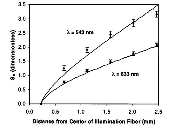

4.1.

Validity and Accuracy

The primary goal of this study was to evaluate the feasibility of our approach to optical property determination in highly attenuating biological media. The computational and experimental (phantom and biological tissue) results presented here all provide strong evidence that this approach is both valid and can achieve at least a moderately high level of accuracy. An initial indication of the validity of the model development algorithms is provided by self-validation results. These cases consistently predicted optical property values with a high level of accuracy, indicating that our MATLAB codes were effective at generating well-calibrated models. An evaluation of the ability of the model to generalize the relationship between S and optical properties beyond the data of the calibration set is provided in the non-self-validation cases, in which simulation data were used for both calibration and evaluation. In these cases, prediction accuracy was good and sometimes even better than for the self-validation case. This indicates that the models were not overly specific to the calibration set, however, other factors, such as the range of the calibration and evaluation dataset may have played a role in determining the RMSE values calculated.

Estimation of tissue phantom optical properties varied significantly with calibration and validation set. As shown in Tables 1 and 2, cases developed with simulation data and evaluated using phantom data tended to have larger RMSE values than those evaluated with simulation data. This is not an unexpected result, since even small experimental errors may have significant impact on the radial reflectance distribution. However, several cases, particularly those developed with the NN approach, indicated low levels of error, approaching ±1 cm ⁻¹ for μ_a and ±2 cm ⁻¹ for μ_s ^′. This level of accuracy provides additional evidence for the validity of this technique and approaches a level that might be adequate to perform highly valuable in vivo measurements.

Since the long-term goal of this research is clinical optical property estimation, data collected on biological tissue provide a reality check that is not possible with computational simulations or tissue phantom measurements. Optical property estimates using our approach and ex vivo bovine liver samples (μ_a=14.5±3.5 cm ⁻¹ and μ_s ^′=7.2±3.7 cm ⁻¹ at 543 nm; μ_a=4.7±1.7 cm ⁻¹ and μ_s ^′=6.7±3.4 cm ⁻¹ at 633 nm) were found to compare favorably with the limited and varied data in the literature. While we are not aware of any data on μ_a for bovine liver at 543 nm, the literature reports a μ_a value of 10.9 cm ⁻¹ for 532 nm and values of 12.0 and 7.9 cm ⁻¹ for porcine liver at 543 and 532 nm, respectively.^{28 29} Given these data, the high blood content of liver, and the 20 increase in blood absorption from 532 to 543 nm,³⁰ it is likely that the true μ_a of bovine liver at 543 nm is only about 10 less than our mean measured value of 14.5 cm ⁻¹ . At 633 nm, the literature indicates μ_a values of 3.0 cm ⁻¹ (Ref. 4) and 3.2 cm ⁻¹ for bovine liver,²⁸ and a μ_a of 5.0 cm ⁻¹ for porcine liver.²⁹ The bovine liver values are about 30 lower than that obtained by our method, though the porcine liver value is almost in exact agreement with our results.

Reduced scattering coefficients of 11.9 cm ⁻¹ for bovine liver at 532 nm,²⁸ and porcine liver values of 10.8 cm ⁻¹ (at 543 nm) and 11.7 cm ⁻¹ (at 532 nm),²⁹ have been determined in prior studies. These values are remarkably consistent and indicate that our measured values may be about 30 lower than expected. Reduced scattering coefficients at 633 nm have been found to be 5.2 cm ⁻¹ for bovine liver²⁸ and 6.4 cm ⁻¹ for porcine liver.²⁹ While these values are in good agreement without μ_s ^′ predictions for bovine liver, both predictions for μ_s ^′ must be viewed as moderately suspect due to their proximity to the lower end of the calibration range. On the whole, our results provide sufficient agreement with the literature as to warrant further evaluation of this technique as a research tool, and after further modification it may be useful for implementation in vivo. However, the present accuracy of this approach is not likely sufficient for many medical diagnostic applications.

One weakness of the present approach is the apparent discrepancy in accuracy between predictions of μ_a and μ_s ^′. The higher RMSE values for μ_s ^′ (Tables 1 and 2) may be explained by the trends seen in Fig. 2. In these graphs it is shown that changes in μ_a have an effect on S that is of greater magnitude than the effect produced by μ_s ^′. Therefore, when the inverse problem of predicting optical properties from S is considered, it follows that any error in S would produce a greater level of error in the estimation of μ_s ^′ than for μ_a. However, improvements in estimation of μ_s ^′ may be possible. Computational modeling results (not shown here) indicated that the intensity of light detected by the first fiber (n=1) is much more highly dependent on μ_s ^′ than on μ_a. By normalizing to the intensity at the first fiber (to minimize error due to variations in illumination intensity), some ability to detect variation in μ_s ^′ is lost. While performing absolute reflectance measurements with an acceptable level of error may be more difficult than our present normalization approach, future research is warranted to evaluate the potential benefits and liabilities of the former technique and optimize the accuracy of μ_s ^′ estimations.

4.2.

Evaluation and Optimization of Model Development

To make progress toward our goal of a clinically useful technique for endoscopic measurement of optical properties in the UVA to VIS region, it is useful to evaluate model performance in terms of the primary independent variables: model type (NN or PLS), data generation approach (modeling or measurement), and optical property distribution (uniform or random). Analysis of the strengths and weaknesses of individual models should lead to advances in experimental and analytical methods.

Estimation accuracy of inverse solution models was dependent on several parameters. Tables 1 and 2 indicate that the most important variable was the type of algorithm used in model generation and calibration. In almost every case, NN models produced lower RMSE values than PLS models, indicating that an NN approach may be a better choice for determination of optical properties. This may be due to the fact that the NN model development algorithm incorporated validation checks using training, testing, and validation sets to avoid overfitting, whereas the PLS code did not contain such checks. Furthermore, PLS develops a linear solution, and therefore may not adequately account for the nonlinear relationships inherent to light transport problems. Calibration of PLS models with independent data points is necessary to create robust models without artifactual correlations. However, our results for PLS model calibration with uniform datasets did not indicate a significant reduction in model quality. While unexpected, this result may be an indication that some factor other than calibration data format—possibly the inherently linear nature of PLS—is the primary factor that limits the efficacy of PLS in this application.

The calibration dataset type also had a strong effect on model quality. In estimating the optical properties of experimental data, NN models calibrated with measured data were slightly more accurate than their simulation-calibrated counterparts. However, self-validation with simulated data produced slightly lower RMSE values than self-validation with experimental data, likely due to experimental error. Since the results found with experimental data calibration were not consistently and significantly better than results for simulation-based calibration, and given the presence of experimental error, we believe that the optimal approach would involve simulation-based calibration.

Several sources of experimental error have been identified. For in vitro measurements, tissue inhomogeneity likely contributed to the variation in the final estimated optical property values. Another source of error may have been the large fiber-to-fiber variation in light intensity, which affected the accuracy of CCD camera measurements. In the future, we plan to homogeneize light levels incident at the CCD through the use of neutral density filters. These and other measurement errors were amplified by the normalization of the radial intensity distributions to the first fiber reading, which may be minimized by using a nonnormalized approach, in which the incident light intensity is strictly regulated and/or determined with a high degree of accuracy.

In general, models calibrated with uniform data produced lower RMSE values than random sets, whereas models validated with uniform datasets produced slightly higher RMSE values than did random sets. This is likely due to the fact that the random dataset included fewer values at the very edge of the μ_a and μ_s ^′ ranges than the uniform set. As a result, increased errors were produced when the model had to evaluate data points that were slightly outside the range it had been trained on. Since the model is most accurate over a restricted range, testing that involves data within this range would produce results more representative of its true accuracy.

One of the most significant limitations of this technique in regards to its eventual use in vivo is its inability to account for layered tissues with different optical properties. If the present techniques were applied to multilayer tissues, such as those found in mucosal tissues of the cervix and esophagus, errors due to different path lengths and relative sampling of the different layers may make it difficult even to obtain accurate estimations of bulk tissue optical properties. However, it may be possible to modify our steady-state reflectance for two-layer tissues, especially if it can be combined with a technique such as optical coherence tomography to provide data on superficial layer thickness.³¹