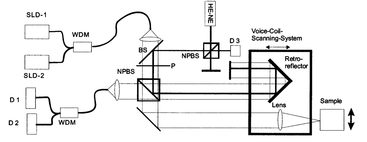
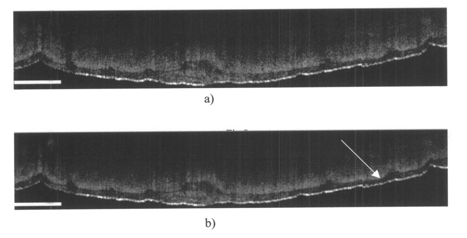
1.IntroductionOptical coherence tomography (OCT), originally developed for cross-sectional imaging of rather transparent ocular tissues,1 2 3 4 5 has found an increasing number of applications in scattering media.6 7 8 9 10 Like other coherent imaging techniques, OCT suffers from speckle noise, which degrades contrast in images of dense biological tissues such as human skin. Several techniques have been introduced to reduce speckle noise, mainly based on spatial compounding11 12 13 or on digital signal-processing algorithms.14 The concept of wavelength compounding was first introduced in the field of OCT by Schmitt et al.;11 However, this method was restricted to compounding of wavelengths contained within the emission spectrum of a single light source, which, as a consequence, reduced longitudinal spatial resolution, a disadvantage that prevented its widespread use in OCT. In this paper we introduce an alternative approach using a frequency compounding-based speckle reduction technique. By the use of two independent light sources with different center wavelengths and emission bands, which do not overlap, we are able to reduce speckle noise. We derive the speckle statistics corresponding to our method and compare the theoretical results with measurements obtained in a uniformly scattering sample. To demonstrate our method in tissue, we recorded images of human skin in vivo and compared the compounded images with those obtained using a single light source. 2.Speckle StatisticsAn early paper on speckle in OCT reported, on an empirical base, grossly similar statistical properties of these speckles compared with those observed in other coherent imaging techniques, if the squared magnitude of the OCT signal is treated as an analog of intensity.11 Later the speckle statistics for a bipolar interferometric OCT signal were mathematically derived.13 This result can, however, not be directly compared with the speckle structure observed in OCT images because the bipolar signal is rectified and low-pass filtered to display only the envelope of the interferometric signal. To describe the speckle observed in OCT images and to compare theoretical results with experimental observations, a modified speckle statistic has to be derived. Speckles arise as a result of a coherent superposition of backscattered light waves from different scattering points or areas of a sample containing densely packed scattering particles. The electromagnetic light waves can be described by a complex-valued phasor represented by amplitude A and phase Φ. Because of random positions of the scattering particles within the coherence length of the illuminating light source and random backscattering potentials, the phasors of waves backscattered from different points can be treated as a random variable, with random amplitude and phase. In the plane of observation we are observing the sum of all phasors. The amplitude A of the phasor sum can be described by a Rayleigh density distribution:15 where σ denotes the standard deviation. The contrast C of a speckle pattern is defined by with σ denoting the standard deviation and A¯ denoting the mean value.15In OCT we observe a sum of two electromagnetic fields—a constant field from the reference arm and a randomly varying field from the sample arm. The field from the sample arm consists of a superposition of fields arising from scattering particles within a coherent volume defined by the coherence length and the illuminated area. The resulting density distribution of the amplitude in the sample arm is given by Eq. (1) when polarized light is used for illumination. Owing to the ac-detection and postprocessing algorithm in OCT systems (rectifying and low-pass filtering), the OCT signal S OCT is given by the real part of the cross-correlation term and therefore is proportional to the amplitudes: where k denotes a constant factor, Ar denotes the constant amplitude from the reference arm, and As denotes the random amplitude of the sample arm varying with depth z, respectively. The corresponding density distribution for the OCT signal is found by performing a transformation of the variables from AS to S OCT via Eqs. (1) and (3).15 This transformation leads to If we calculate the mean value of this distribution, we find the relationship where S¯ OCT denotes the mean value of the OCT signal. Substituting Eq. (5) in Eq. (4) leads to the density distribution of the OCT signal for polarized light: This is a Rayleigh density distribution and therefore has a speckle contrast of 0.52.The same result is obtained if we treat Eq. (3) as a change of scale, which changes the mean value but not the shape of the density distribution. If we incoherently superimpose two speckle fields with distributions given by Eq. (6), for example by use of nonpolarized light or two uncorrelated light sources with different center wavelengths, the new density distribution is given by a convolution of two independent density distributions,15 each of the form given by Eq. (6): Via the second moment of this distribution we obtained a speckle contrast of 0.36, which corresponds to a speckle contrast reduction of 1.4 in comparison with Eq. (6).Melton and Magnin16 proposed that the cross-correlation coefficient between fully developed speckle patterns formed in two Gaussian frequency bands of equal width with center frequencies separated by fs is given by where ρxy denotes the cross-correlation between the frequency band centered at x and the frequency band centered at y, and B denotes the full width at half maximum (FWHM) of each band. This equation may be written in terms of the FWHM of the emission spectrum of the light source Δλ, and the wavelength difference λs (assuming the same Δλ for both light sources): Therefore, two independent light sources with different center wavelengths and spectral emissions that do not overlap have a correlation coefficient rapidly approaching zero with increasing wavelength difference. In other words, the speckle fields of the two light sources are uncorrelated if the difference of the center wavelengths is large enough. There is an alternative definition of the cross-correlation coefficient ρ(0,0) (at zero displacement between the two speckle fields), which gives us an important measure of the correlation between two speckle fields15 where u(v) denotes the intensity in a point of the speckle field arising from the first (second) light source and u¯(v¯) denotes the mean intensity.3.MethodOur method is based on a compounding of two wavelengths. The scheme of the experimental setup is shown in Fig. 1. It consists of two single-mode, fiber-coupled superluminescent diodes (SLDs), with the center wavelengths at 1312 nm (FWHM bandwidth Δλ=36 nm) and at 1488 nm (FWHM bandwidth Δλ=57 nm) , respectively. The corresponding round-trip FWHMs of the source intensity coherence envelopes17 are 21 and 17 μm, respectively. The two light sources are combined by a wavelength division multiplexer (WDM). The emitted light beams of SLDs used here are partially polarized. To eliminate the influence of partially polarized light on our measurements, we place a polarizer into the beam before the dual-wavelength beam is coupled into a free-space interferometer, where it is split by the nonpolarizing beamsplitter into a reference beam and a sample beam. The reference beam is folded by a retroreflector and backreflected by a mirror. The sample beam is focused on the sample by a lens that is mounted on the same translation stage as the retroreflector. This setup provides dynamic focusing.18 The light in the sample arm is backscattered by the sample and collimated by the lens. The nonpolarizing beamsplitter recombines the reference and sample beam. The recombined beam is coupled into a single-mode fiber, and a wavelength division multiplexer separates the two wavelengths. Separate detectors measure the interference patterns corresponding to the two wavelengths that arise from the superposition of sample and reference light independently. By moving the translation stage with a constant velocity, a Doppler shift of the reference beam is introduced, causing a heterodyne interferometric signal centered at the Doppler frequency. This enables measurements with high sensitivity. The electric signals are amplified, corrected for nonlinearities of the translation stage (see Sec. 4), digitally bandpass filtered, and rectified. The signal envelopes are displayed on a logarithmic gray-scale map. The sensitivity of our system was measured with 94 dB, at an A-scan rate of 8 A-scans per second. To eliminate nonlinearities in scanning speed, an auxiliary interferometer with a long-coherence He-Ne laser was added to the experimental setup. The interferometric signal arising from the He-Ne laser was used to measure the instantaneous velocity of the scanning stage, and this information was used to numerically correct nonlinearities of the velocity. 4.ResultsThe first aim of our study was to investigate the speckle statistics of the OCT image. For an optimum speckle reduction, it is necessary to ensure that the two speckle patterns recorded with the two light sources are statistically uncorrelated. The ideal test sample for generating randomly distributed speckle patterns should be uniformly scattering, should have no internal structure on a scale larger than coherence length, and should be nonabsorbing at the two wavelengths. After experiments with different materials, we choose a piece of plastic rubber as the scattering test sample. Speckle patterns were obtained by recording OCT tomograms consisting of 400 A-scans with a transversal step size of 2.5 μm, resulting in a total transversal scan of 1000 μm (focus beam diameter ≈10 μm) . The depth sampling interval and total sampling depth were 0.05 and 2500 μm, respectively. After rectifying and low-pass filtering, the data sets were reduced in depth by a factor of 20. The OCT images of the sample are shown in Fig. 2. Figure 2OCT images of a uniformly scattering test sample (plastic rubber). (a) 1488 nm, (b) 1312 nm (the arrow indicates the direction of illumination). 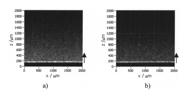 To compare the experimental results with theory, it is necessary to correct for the exponential decay with depth in OCT signals. This can be done in several ways. The simplest way, which was used in this investigation, is to take the logarithm of the signal and to perform a linear fit. We minimized the influence of speckle noise on the result of this fitting procedure by averaging over 200 A-scans before fitting. The slope of this fit is then used to recalculate the backscattered intensities. Figure 3 shows the logarithmic intensities of the averaged A-scans and the corresponding linear fit and the corrected signal. Figure 3Averaged logarithmic OCT signals (solid line), linear fit (dashed line), and recalculated signal (dotted line). 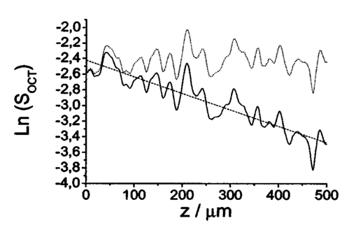 To investigate the correlation between the speckle patterns recorded at the two wavelengths, we calculated the cross-correlation coefficient ρ for different subsections and different subsection sizes of the OCT images. For optimum speckle reduction, the cross-correlation coefficient should be zero. As shown in Fig. 4, the correlation coefficient is very small. The fluctuations for window sizes smaller than 50×50 μm 2 result from the small numbers of pixels within the windows, and therefore random intensity correlations have a large impact on the result. The low correlation coefficient for larger-sized subsections indicates that the speckle fields are essentially uncorrelated. Figure 5 shows an example of a 500×500-μm large subsection of Fig. 2. Figure 4Variation of the cross-correlation coefficient ρ of the speckle patterns recorded at the two wavelengths with increasing subsection size; s, side length of the quadratic subsection. 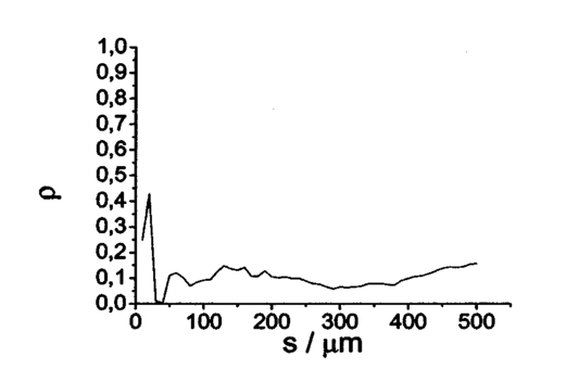 Figure 5Example of a subsection (500×500 μm) of the OCT images from Fig. 2. (a) Subsection of the 1312-nm image, (b) subsection of the 1488-nm image. 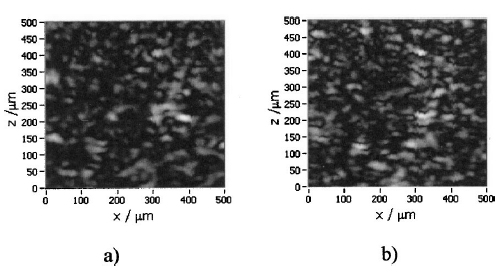 Figure 6 is a comparison of the intensity distribution according to Eq. (6) with the intensity distributions obtained from Fig. 5. The experimental data show good agreement with the theoretical values. The speckle contrast C was measured from Fig. 5(a) to 0.625 and from Fig. 5(b) to 0.637, respectively. For speckle reduction, the OCT intensity images of Figs. 2(a) and 2(b) were added incoherently, i.e., the envelopes of the OCT signals were added. Figure 7 shows a subsection of the compounded image (an area similar to that in Fig. 5) and the corresponding theoretical [Eq. (7)] and experimental intensity probability distributions. The slight mismatch between the experimental data and the theoretical values probably results from the residual correlation (ρ≈0.2) between the images of the two wavelengths, which may be caused by larger structures of the sample. From theory we expect a decrease in speckle contrast by a factor of 1.4, but the measured decrease of the speckle contrast from Fig. 7(a) is by a factor of 1.25. We believe that the residual correlation between the speckle fields is responsible for this mismatch (a residual correlation caused by larger sample structures gives rise to speckles whose positions are correlated to some degree with the sample structure; therefore these speckles are less effectively reduced by a method based on uncorrelated speckle fields). Figure 6Probability distribution of the speckle intensity values in Fig. 5. Solid line, theoretical values according to Eq. (6); data points; measured values. 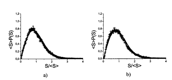 Figure 7(a) The compounded image of the subsection from Fig. 5(b) Probability distribution of the speckle intensity from (a). Solid line, theoretical values; data points; measured values.  To demonstrate our method in real tissue, we recorded OCT images in human skin across a scar of a fingertip in vivo. Figure 8 shows the result. This tomogram consists of 1900 A-scans with a lateral step size of 5 μm. To reduce the intensity of the reflex from the skin surface, we applied glycerine to the surface (index matching). Figure 8(a) shows a raw image obtained at a single wavelength (1312 nm); Fig. 8(b) shows the compounded image. The different layers show more contrast in the compounded image; in particular the border between the stratum corneum and stratum spinosum [indicated by an arrow in Fig. 8(b)] is more visible. In the center of the image, directly below the surface, the structural damage corresponding to the scar can be seen. Within the scar area, small structures appear better separated in the compounded image than in the single-wavelength image, whereas regions with nonresolvable structures appear smoothed in the compounded image [for a visible recognition of these features, high-quality prints are necessary; the improvement of image quality in Fig. 8(b) is best observed by viewing the image files provided in the online version of this journal]. To quantify the improvement of the compounded image, we calculated the speckle contrast in five different regions [(an area 500×500 μm 2) of Figs. 8(a) and 8(b)]. The speckle contrasts in the five regions were averaged, and the compounded image showed an average reduction in the speckle contrast by a factor of 1.25 compared with the image recorded at a single wavelength. This corresponds to an improvement in the signal to noise ratio of (1.25)2≈1.56. 5.ConclusionsWe derived the speckle statistics for OCT systems and compared the theoretical results with data obtained by a uniformly scattering test sample. These results show a good agreement with the theoretical predictions. We investigated and demonstrated, to our knowledge for the first time, a frequency compounding method with the use of two different light sources for speckle reduction in optical coherence tomography. An application of our method to imaging of human skin demonstrated a visible increase in image quality. One drawback of the method is the increased complexity of the system. This complexity is further increased if more than two light sources are compounded, which would be necessary for further reduction of speckle noise. The main advantage of this method, compared with other speckle reduction techniques, lies in the fact that spatial resolution is maintained. Another advantage is that the same system can be used to perform differential absorption measurements if the sample contains substances of different absorption coefficients at the two wavelengths. AcknowledgmentsThe authors wish to thank H. Sattmann and L. Schachinger for technical assistance. Financial assistance from the Austrian Fonds zur Fo¨rderung der wissenschaftlichen Forschung (grant P14103-MED) is acknowledged. REFERENCES
D. Huang
,
E. A. Swanson
,
C. P. Lin
,
J. S. Schuman
,
W. G. Stinson
,
W. Chang
,
M. R. Hee
,
T. Flotte
,
K. Gregory
,
C. A. Puliafito
, and
J. G. Fujimoto
,
“Optical coherence tomography,”
Science (Washington, DC, U.S.) , 254 1178
–1181
(1991). Google Scholar
A. F. Fercher
,
C. K. Hitzenberger
,
W. Drexler
,
G. Kamp
, and
H. Sattman
,
“In vivo optical coherence tomography,”
Am. J. Ophthalmol. , 116 113
–114
(1993). Google Scholar
W. Drexler
,
U. Morgner
,
F. X. Kaertner
,
C. Pitris
,
S. A. Boppart
,
X. D. Li
,
E. P. Ippen
, and
J. G. Fujimoto
,
“In vivo ultrahigh-resolution optical coherence tomography,”
Opt. Lett. , 24 1221
–1223
(1999). Google Scholar
A. G. Podoleanu
,
G. M. Dobre
,
D. J. Webb
, and
D. A. Jackson
,
“Simultaneous en-face imaging of two layers in the human retina by low-coherence reflectometry,”
Opt. Lett. , 22 1039
–1041
(1997). Google Scholar
A. Baumgartner
,
C. K. Hitzenberger
,
H. Sattmann
,
W. Drexler
, and
A. F. Fercher
,
“Signal and resolution enhancements in dual beam optical coherence tomography of the human eye,”
J. Biomed. Opt. , 3 45
–54
(1998). Google Scholar
G. J. Tearney
,
M. E. Brezinski
,
B. E. Bouma
,
S. A. Boppart
,
C. Pitris
,
J. F. Southern
, and
J. G. Fujimoto
,
“In Vivo Endoscopic Optical Biopsy with Optical Coherence Tomography,”
Science (Washington, DC, U.S.) , 276 2037
–2039
(1997). Google Scholar
J. De Boer
,
Z. Chen
,
J. S. Nelson
,
S. Srinivas
, and
A. Malekafzali
,
“Imaging thermally damaged tissue by polarization sensitive optical coherence tomography,”
Opt. Express , 3 212
–218
(1998). Google Scholar
F. I. Feldchtein
,
D. Reitze
,
A. Sergeev
,
V. Gelikonov
,
G. Gelikonov
,
R. Kuranov
,
N. Gladkova
,
R. Iksanov
,
M. Ourutina
, and
J. Warren
,
“In vivo OCT imaging of hard and soft tissue of the oral cavity,”
Opt. Express , 3 239
–250
(1998). Google Scholar
A. Rollins
,
J. Izatt
,
M. Kulkarni
,
S. Yazdanfar
, and
R. Ung-arunyawee
,
“In vivo video rate optical coherence tomography,”
Opt. Express , 3 219
–229
(1998). Google Scholar
A. Baumgartner
,
S. Dichtl
,
C. K. Hitzenberger
,
H. Sattmann
,
B. Robl
,
A. Moritz
, and
A. F. Fercher
,
“Polarisation-sensitive optical coherence tomography of dental structures,”
Caries Res. , 34 59
–69
(2000). Google Scholar
J. M. Schmitt
,
S. H. Xiang
, and
K. M. Yung
,
“Speckle in optical coherence tomography,”
J. Biomed. Opt. , 4 95
–105
(1999). Google Scholar
J. M. Schmitt
,
“Array detection for speckle reduction in optical coherence microscopy,”
Phys. Med. Biol. , 42 1427
–1439
(1997). Google Scholar
M. Bashkansky
and
J. Reintjes
,
“Statistics and reduction of speckle in optical coherence tomography,”
Opt. Lett. , 25 545
–547
(2000). Google Scholar
H. E. Melton
and
P. A. Magnin
,
“A-mode speckle reduction with compound frequencies and compound bandwiths,”
Ultrasound Imag. , 6 159
–173
(1984). Google Scholar
E. A. Swanson
,
D. Huang
,
M. R. Hee
,
J. G. Fujimoto
,
C. P. Lin
, and
C. A. Puliafito
,
“High-speed optical coherence domain reflectometry,”
Opt. Lett. , 17 151
–153
(1992). Google Scholar
J. M. Schmitt
,
S. L. Lee
, and
K. M. Yung
,
“An optical coherence microscope with enhanced resolving power in thick tissue,”
Opt. Commun. , 142 203
–207
(1997). Google Scholar
|


CITATIONS
Cited by 255 scholarly publications and 38 patents.
Optical coherence tomography
Speckle
Light sources
Scattering
Beam splitters
Light scattering
Speckle pattern


