1.

Introduction

Recently there has been increased interest in the propagation of polarized light in randomly scattering media, such as biological tissues, because of its potential applications, particularly in biomedical imaging and diagnosis. Optical technology offers significant advantages for imaging human tissues because it employs nonionizing radiation and provides a high contrast between early cancers and the background normal tissues. However, the random scattering of light in biological tissues deteriorates the imaging resolution, which presents the main challenge associated with optical imaging. Ultrafast optics can be used to enhance optical imaging and diagnosis. With this technique, a short light pulse is applied to the biological tissues, and then the transmitted ballistic and quasi-ballistic photons that carry more information about biological tissue properties are extracted through various gating techniques. Since multiply scattered photons usually have longer path lengths than weakly scattered photons, they can be excluded by time gating.^{1 2 3 4 5} Polarization gating can be used as an alternative method for extracting the ballistic and quasi-ballistic components because weakly scattered light preserves its original polarization better than multiply scattered light.^{6 7 8 9 10} Polarization propagation in biological tissues is a complicated process that is fundamental to tissue optics. Many parameters, such as size, shape, refractive index, concentration of the scattering particles, and incident polarization state play important roles in the scattering of light.^{11 12}

In order to improve the quality of optical imaging using ultrafast light sources, more study is necessary to fully understand the evolution of the polarization state in scattering media, as well as the time- and polarization-dependent distribution of light transmitted through the media. The Monte Carlo (MC) technique offers a flexible and accurate approach to these problems, since it can trace detailed information in polarization propagation inside and outside a scattering medium with complex geometries and can score multiple physical quantities simultaneously.^{13 14}

By employing a streak camera and an ultrafast laser source, in this study we analyze the temporal profiles of the Stokes components of light transmitted through scattering media made of polystyrene-microsphere solutions, where the incident light pulses are linearly polarized and circularly polarized, respectively. A time-resolved MC technique based on the Stokes-Mueller formalism is developed to analyze polarization propagation through these scattering media. The polarization distributions after a single scattering and after multiple scatterings are compared and discussed. The MC-simulated Stokes vectors of transmitted light are compared with the measurements obtained in experiments. We study and explain some of the properties of the polarization-dependent time-resolved transmitted light that can be observed from the experimental and MC results. Polystyrene-microsphere solutions with various particle diameters and scattering concentrations have been studied. Here we present the results for 380-nm polystyrene-microsphere solutions with scatterer concentrations of 0.133 and 0.066.

2.

Experimental Setup

The experimental setup is shown in Fig. 1. A titanium:sapphire (Ti:sapphire) laser is used to provide 800-nm light pulses with a FWHM of 100 fs. The laser beam is split into two branches, one for triggering the streak camera and the other for propagating through the scattering media. An average power of 200 mW is applied to the input surface of the media. The incident polarization state is controlled by a polarizer, a zero-order half-wave plate, and a zero-order quarter-wave plate. Meanwhile, the detected polarization state is controlled by a zero-order quarter-wave plate and a linear analyzer. The light transmitted from the scattering media is directed to the streak camera with a fiber bundle. The diameter of the receiving area is 1 mm, and the receiving angle of the fiber bundle is about 30 deg. The temporal resolution of the operational mode of the streak camera is 4.74 ps. Because of the dispersion of the optical signal in the fiber bundle and the limited resolution of the streak camera, the response of the detection system to the laser pulse has a FWHM of 20 ps, as shown by the normalized profile in Fig. 1(b).

Figure 1

(a) The schematic diagram of the experimental setup, where P is a polarizer, HW is a zero-order half-wave plate, QW is a zero-order quarter-wave plate, and A is a linear analyzer. (b) The response of the detection system to the laser pulse.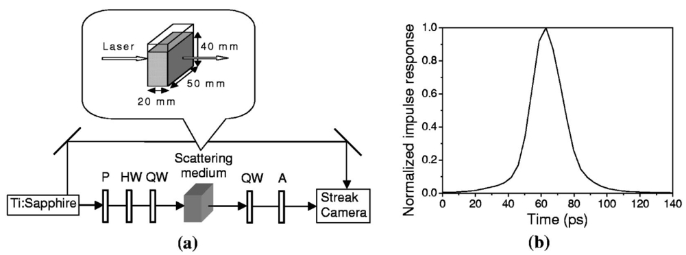

The scattering media are composed of polystyrene-microsphere solutions contained in a transparent plastic cubic cuvette, with a size of 5×5×2 cm, where L, the thickness of the cuvette along the laser axis, is 2 cm. The polystyrene-microsphere solutions occupy the cuvette to about 80 of the volume. The absorption coefficient of the solutions is low enough to be regarded as zero. The polystyrene microspheres have a diameter 2a of 380 nm±13 nm. The refractive indices of the background medium, n_b, and the polystyrene microspheres, n_s, are 1.329 and 1.565, respectively, at a wavelength (λ) in vacuo of 800 nm. The speed of light, c, in the scattering media is 0.0226 cm/ps. The polystyrene-microsphere solution is diluted to different concentrations to achieve different scattering mean-free-paths (SMFP), l_s. The incident laser beam enters the medium from the center of the input surface. The fiber bundle and the incident beam are aligned with each other so that the area detected on the output surface of the medium has a circular symmetry about the axis of the incident light.

3.

Monte Carlo Analysis

The geometry of multiple scattering events in a polystyrene-microsphere solution is shown in Fig. 2(a). The MC simulation that describes the multiple scattering events of light in turbid media is based on radiative theory, which assumes that scattering events are independent and ignore coherent effects. A narrow pencil beam propagates downward along the z-axis into a plane-parallel slab of scattering medium with a thickness of L. The incident point is (0, 0, 0) in the laboratory coordinate system (x, y, z). Photon packets are scattered in the medium by microspheres before exiting the upper or lower surface of the medium. At each scattering event, the scattering angles of the photon packets are statistically selected according to Mie theory.¹⁵ During propagation, the polarization evolutions of photon packets are traced through the Stokes-Mueller formalism.^{16 17}

Figure 2

(a) The geometry of multiple scattering events in a slab of turbid medium. (b) The geometry of the first scattering event during light propagation.

To begin, we analyze the first scattering event that the photon packets encounter after they enter the input surface of a scattering medium. The scattering geometry is shown in Fig. 2(b), where Θ∈[0,π] is the polar angle between the propagation orientations before and after the scattering, and ϕ∈[0,2π) is the azimuthal angle between the reference plane and the scattering plane. Once Θ and ϕ are known, the propagation orientation after the scattering is determined. The Stokes vector of light after the first scattering event can be expressed as

For an 800-nm light scattered by 380-nm-diameter polystyrene microspheres, the size parameter, ka=2πn_ba/λ, is 2.0 and the light scattering is in the Mie regime. The three-dimensional distributions of the Stokes vectors S ₁ for the H and R incident polarization states are shown in the left columns in Fig. 3 and Fig. 4, respectively. The intensity distributions of S ₀ are normalized at the peak point where the polar angle Θ=0. Patterns of S ₁/S ₀, S ₂/S ₀ and S ₃/S ₀ show the comparative intensity distribution of the Stokes components with respect to S ₀.

Figure 3

(Left column) Three-dimensional distributions of the Stokes components of light after a single scattering event and (right column) the spatial patterns of the Stokes components of light transmitted through a slab of turbid medium, where the incident light is linearly polarized with the orientation of polarization along the x-axis; S ₁, S ₂, and S ₃ are normalized with respect to the intensity distribution S ₀.

Figure 4

(Left column) Three-dimensional distributions of the Stokes components of light after a single scattering event and (right column) the spatial patterns of the Stokes components of light transmitted through a slab of turbid medium, where the incident light is right circularly polarized; S ₁, S ₂, and S ₃ are normalized with respect to the intensity distribution S ₀.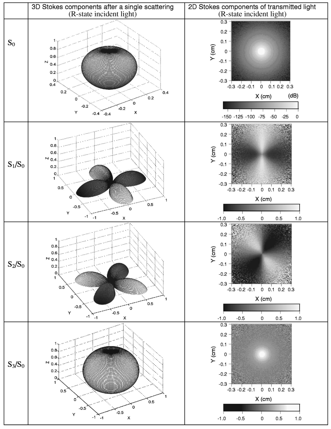

For both the H and R incident polarization states, all of the light energy propagates forward (0⩽Θ<45 deg) after a single scattering event. The integral of S ₀ along the azimuthal angle ϕ leads to the intensity distribution as a function of the polar angle Θ, which is constant for any incident polarization state. For the H incident state, the Stokes components S ₀ and S ₁ depend on the azimuthal angle ϕ from 0 to 2 π, while for the R incident state, the Stokes components S ₀ and S ₃ are independent of ϕ. The Stokes components S ₂ and S ₃ for H, and S ₁ and S ₂ for R, have cloverleaflike patterns projected on the x-y-plane, as shown in Fig. 3 and Fig. 4. The two positive leaves (bright leaves) and the two negative leaves (dark leaves) in each pattern are symmetrically distributed around the center point.

Using the Stokes-Mueller formalism, we trace the evolution of the polarization state of each photon packet through the successive multiplication of the matrices M(Θ) and R(ϕ). The detailed method for tracing the photon propagation was based on an idea in Ref. 18. The Stokes vector, S _n ^fs, of a transmitted photon packet that has been scattered n times by spherical scattering particles in a turbid medium can be briefly expressed as

The spatial patterns of the transmitted Stokes components for the H and R incident polarization states are shown in the right columns in Fig. 3 and Fig. 4, respectively, where the thickness L of the 380-nm polystyrene-microsphere solutions is 1 cm, the anisotropic factor g is 0.65, the scatterer concentration is 0.066, the scattering coefficient μ_s is 4.61 cm ⁻¹ , and the absorption coefficient μ_a is set to be 0. The SMFP and the factor L/l_s are simulated to be 0.22 cm and 4.61, respectively. Each pattern in the x-y plane shows a 0.6×0.6 cm area on the output surface of the scattering medium. To make the spatial patterns of S ₀ clearer, we show the decibel values of the intensities. Other Stokes components, S ₁, S ₂, and S ₃, for each position are normalized with S ₀. The patterns of transmitted Stokes components show different preferential orientations, which are mainly determined by incident polarization states. According to Eqs. (5) to (7), the integral values of the intensity S ₀ in any circular area centered at the axis of the incident light are the same for the H and R incident polarization states, although the intensity distributions of S ₀ for the H and R states show different preferential orientations.

The remaining degree of polarization (DOP) and the patterns of the Stokes vectors of transmitted light come from the lowly scattered photon packets. Considering a scattering medium with a greater factor of L/l_s, the ratio of lowly scattered light in the total transmitted light is lower. Therefore, the remaining DOP and the spatial patterns of the Stokes vectors are weaker. However, the shapes of the patterns of the Stokes components remain the same for scattering media with different factors of L/l_s. Our MC-simulated polarization patterns of transmitted light are similar to the experimental and analytical results obtained by previous researchers.^{19 20 16 13}

We can see in Fig. 3 and Fig. 4 that projections of the 3-D patterns after single scattering events on the x-y-plane lead to 2-D polarization distributions that match well with the corresponding 2-D patterns of the transmitted Stokes components. This demonstrates that the key features of 2-D spatially distributed polarization of light, transmitted through a scattering medium containing spherical particles, are determined by the first scattering event that the light encounters, while the background level in the polarization pattern is affected by the multiply scattering events.

In time-resolved measurements of transmitted Stokes components, the incident beam and the fiber bundle for detection are aligned with each other. The detected Stokes components come from the integral of the transmitted photon packets in the detection area ((x²+y²)^1/2<0.5 mm) centered at the (0, 0) point in the x-y-plane. We expect that the signals of S ₂ and S ₃ for the H incident polarization state, and S ₁ and S ₂ for the R incident polarization state will be zero, because in the patterns of these Stokes components, the positive leaves and negative leaves are distributed symmetrically in respect to the center. Therefore, for the H and R incident polarization states, the DOP of transmitted light comes entirely from Stokes components S ₁ and S ₃, respectively. When the detection area is not centered at the (0, 0) point, these Stokes components, S ₂, S ₃ for the H and S ₁, S ₂ for the R, may not be zero and their values are highly dependent on the detection area on the x-y-plane.

Depending on the length of the propagation paths, the transmitted photon packets are recorded in different units in the time space. Since the incident photons are launched simultaneously, we convolute the temporal profiles of the transmitted Stokes vectors with the response of the detection system to the laser pulse to match the experimental measurements. The time-resolved transmitted Stokes vector has the form

4.

Time-Resolved Results and Discussion

In the following results, the 0 point on the time axis depicts the time when the light is received by the detector after it transmits the cuvette with water. Therefore the time when the incident light pulse enters the scattering medium is −L/c, which equals −88.6 ps when the thickness L of the slab is 2 cm. The temporal profiles of the Stokes components of transmitted light have been normalized with respect to the maximum value of S ₀, which makes the comparison between the MC simulations and experimental measurements possible.

For a 380-nm polystyrene-microsphere solution with a concentration of 0.133, the scattering coefficient μ_s and the anisotropic factor g are simulated to be 9.22 cm ⁻¹ and 0.65, respectively. The SMFP, l_s, and the factor L/l_s are 0.11 cm and 18.44. The time-resolved Stokes components S ₀ and S ₁ and the DOP of the transmitted light when the incident light is H state polarized are shown in Figs. 5(a), 5(b), and 5(c), respectively. The FWHM of S ₀ is 208 ps. The maximum intensity of S ₁ is 0.43. The time-resolved Stokes components S ₀ and S ₃ and the DOP of the transmitted light when the incident light is R state polarized are shown in Figs. 5(d), 5(e), and 5(f), respectively. The FWHM of S ₀ is 206 ps. The maximum intensity of S ₃ is 0.58. For both the linearly and circularly incident polarization states, the experimental results (scattered circles), including the Stokes components and the DOP, match well with the results from the MC simulations (solid lines). In Fig. 5, the Stokes components S ₂, S ₃ for the H incident state and S ₁, S ₂ for the R incident state are not presented because they show very weak values compared with the intensities of S ₀ and can be regarded as zero. This phenomenon can be explained by considering the symmetrical patterns of these Stokes components and the circular symmetrical distribution of the detection area around the axis of the incident laser beam, which was discussed in Sec. 3.

Figure 5

Time-resolved Stokes components S ₀ (a) and S ₁ (b) and degree of polarization (c) of transmitted light where the incident light is linearly polarized. Time-resolved Stokes components S ₀ (d) and S ₁ (e) and degree of polarization (f) of transmitted light where the incident light is circularly polarized. The scattering medium is a 380-nm polystyrene-microsphere solution with a scatterer concentration of 0.133. The circles depict the experimental measurements and the solid lines show the MC simulations. The dashed lines in (a) and (d) show the simulation results based on the diffusion model. The order of scatters as functions of the propagation time is also shown as dashed lines in (c) and (f) for linearly and circularly incident polarization states, respectively.

It can be observed that for linearly and circularly incident polarization states, the time-resolved profiles of S ₀ of transmitted light are similar, which shows that the temporal distribution of the light transmittance is independent of the incident polarization state. According to our detection system, S ₀ is the integral of the light intensity within the detection area that is a circular area centered at the (0, 0) point on the x-y-plane. As shown in Sec. 3, although the spatial patterns of S ₀ are different for various incident polarization states, the total light energies that enter the detection area are the same. We know that the trajectories of the photon packets in the turbid medium are determined by both the PDF of polar angle Θ and the PDF of azimuthal angle ϕ in successive single scattering events. However, by considering the circular symmetrical distribution of the detection area around the incident light axis, we can deduce that the detected temporal profile of S ₀ is independent of the PDF of ϕ but totally determined by the PDF of Θ in successive single scattering events. Moreover, as we have discussed, the intensity distribution as a function of the polar angle Θ after a single scattering is independent of the polarization state. Therefore, with the detection geometry in the experiment, the detected temporal profiles of S ₀ of the transmitted light are the same for various incident polarization states.

By employing the radiative transfer theory based on the diffusion approximation,²¹ we simulate the temporal profiles of light transmittance through a slab of turbid medium to compare with the results from the MC simulations and the experiments. Accurate results can be obtained when the two conditions in Eq. (11) are satisfied:

We convolute the time-dependent transmittance based on the radiative transfer theory with the response of the detection system to the laser pulse to simulate the S ₀ profile measured in the experiments, which are shown in Figs. 5(a) and 5(d) with the dashed curves normalized at the peak value. The results from the diffusion model match the MC simulation and the experimental results well after 250 ps. At times before 250 ps, there is considerable discrepancy between them because the photons exiting the scattering medium at an earlier time have not encountered multiple scattering and the distribution of their propagations is not adequately isotropic to be described by diffusion theory.

The MC-simulated average order of scatters, 〈N〉, as a function of the light propagation time are shown in Figs. 5(c) and 5(f) as dashed lines. After about 20 ps, 〈N〉 shows a good linear relationship with the propagation time, which can be expressed as

Figures 5(c) and 5(f) show that for both linear and circular incident polarization states, the DOP of the transmitted light with respect to the propagation time decays exponentially after about 20 ps when 〈N〉 is greater than 16. In a previous publication, Bicout et al.;¹¹ presented the exponential relationship between the DOP of light and the factor d/l_s for the forward propagation mode, where d is the thickness of the turbid medium. Ambirajan and Look²² found that the degree of linear polarization of backward-scattered light decreases exponentially with respect to the order of scatters. Because of the linear relationship between 〈N〉 and the propagation time of the light, the exponential decay of the DOP of the transmitted light as a function of time can be explained.

For a 380-nm polystyrene-microsphere solution with a concentration of 0.066, the scattering coefficient μ_s is 4.61 cm⁻¹, the SMFP l_s is 0.22 cm, and the factor L/l_s is 9.22, which is half that of the 0.133 solution. The time-resolved Stokes components S ₀ and S ₁ and the DOP of the transmitted light when the incident light is linearly polarized are shown in Figs. 6(a), 6(b), and 6(c), where the FWHM of S ₀ is 22 ps, the maximum S ₁ is 0.97, and the FWHM of the DOP is 62 ps. The time-resolved Stokes components S ₀ and S ₃ and the DOP of the transmitted light when the incident light is circularly polarized are shown in Figs. 6(d), 6(e), and 6(f), where the FWHM of S ₀ is 20 ps, the maximum S ₃ is 0.98, and the FWHM of the DOP is 71 ps. The experimental results (scattered circles) matched well with the MC simulations (solid lines) for this 0.066 polystyrene–microspheres solution.

Figure 6

Time-resolved Stokes components S ₀ (a) and S ₁ (b) and degree of polarization (c) of transmitted light, where the incident light is linearly polarized. Time-resolved Stokes components S ₀ (d) and S ₁ (e) and degree of polarization (f) of transmitted light where the incident light is circularly polarized. The scattering medium is a 380-nm polystyrene-microsphere solution with a scatterer concentration of 0.066. The circles depict the experimental measurements and the solid lines show the MC simulations. The dashed lines in (a) and (d) show the simulation results based on the diffusion model. The order of scatters as functions of the propagation time is also shown as dashed lines in (c) and (f) for linearly and circularly incident polarization states, respectively.

The FWHM of S ₀ for this 0.066 solution is less than that for the 0.133 polystyrene-microsphere solution, regardless of the incident polarization state. Because of the lower scattering coefficient of this medium, the percentage of lowly scattered light in the total transmittance is higher. Most transmitted light comes from the ballistic and quasi-ballistic component, which has a comparatively shorter duration than highly scattered light. Therefore the intensity of S ₀ in Fig. 6 decreases much faster than that for the 0.133 solution. Moreover, since the main part of S ₀ comes from the ballistic and quasi-ballistic component, the simulation result (dashed lines) based on the diffusion model does not fit with the profiles measured in experiments.

In Figs. 6(c) and 6(f), the temporal profiles of the DOP decay exponentially for both linearly and circularly incident polarization states. The DOP of the light transmitted through the 0.066 polystyrene-microsphere solution decays more slowly compared with the results for the 0.133 solution. This is not surprising since light propagating through this medium with a lower scattering coefficient encounters fewer scattering events during the same propagation length. Similarly to the 0.133 solution, the 〈N〉 of light transmitted through this solution also shows a linear relationship with respect to the propagation time after 25 ps. For this solution, the slope of the 〈N〉 as a function of time is half that for the 0.133 solution because its SMFP is double that for the 0.133 solution.

For initially polarized light transmitted through the 380-nm polystyrene-microsphere solutions, the average order of scatters 〈N〉 at the time when the DOP decreases from 1 to 0.5 is more than 10, which is obviously greater than that observed for backscattered light.^{11 23 24} Compared with the backscattered light, the transmitted light in its early stage of propagation encounters mainly forward scattering events with small scattering angles. Because the DOP attenuation for small-angle scattering events is weaker than that for large-angle scattering events, it follows that the transmitted light keeps its polarization state better than the backscattered light.

5.

Conclusion

A time-resolved MC technique based on the Stokes-Mueller formalism is employed in this study of initially polarized ultrafast laser pulse propagation through 380-nm polystyrene-microsphere solutions with different concentrations. Simulated temporal profiles of the Stokes components and the DOP are compared with the measurements obtained in experiments that employ a streak camera with a 4.74-ps resolution. A satisfactory match between them proves the accuracy of this MC algorithm. The correlation between the 3-D Stokes components of light after the single scattering event and the spatial distribution of the Stokes components on the output surface of the turbid medium shows that the polarization patterns of transmitted light are mainly determined by the first scattering event that the light encounters during propagation. The spatial distribution of the transmitted intensity is dependent on the polarization state of the incident light, which can be forecast through the PDF of the azimuth angle ϕ in the first scattering event. When the detection area has a circular symmetrical distribution around the axis of the incident light, the temporal profile of transmittance is independent of the incident polarization state but is determined mainly by the PDF of the polar angle Θ in successive single scattering events. By considering the linear relationship between the average order of scatters and the light propagation time, we can interpret the exponential decay of the DOP of the transmitted light with respect to the propagation time.

Compared with the diffusion model, simulations based on the MC technique present a more precise match with the experimental measurements, especially when lowly scattered light is the dominating component in the total transmittance. In addition to the propagation of light intensity, the MC simulation based on the Stokes-Mueller formalism presents detailed information on the evolution of polarization in turbid media. This can help us understand the phenomena observed in laser–tissue interactions and can potentially help us improve the quality of optical imaging that utilizes time gating or polarization gating techniques. Because of the nature of the MC simulation, coherent phenomena cannot be modeled. However, this simulation method can be applied in the noncoherent regime or in cases where the coherent effects are removed.