Radiative transport in the delta-P1 approximation: accuracy of fluence rate and optical penetration depth predictions in turbid semi-infinite media

Stefan A. Carp; Scott A. Prahl; Vasan Venugopalan

doi:10.1117/1.1695412

1 May 2004 Radiative transport in the delta-P1 approximation: accuracy of fluence rate and optical penetration depth predictions in turbid semi-infinite media

Stefan A. Carp, Scott A. Prahl, Vasan Venugopalan

Author Affiliations +

Journal of Biomedical Optics, Vol. 9, Issue 3, (May 2004). https://doi.org/10.1117/1.1695412

Abstract

Using the δ-P₁ approximation to the Boltzmann transport equation we develop analytic solutions for the fluence rate produced by planar (1-D) and Gaussian beam (2-D) irradiation of a homogeneous, turbid, semi-infinite medium. To assess the performance of these solutions we compare the predictions for the fluence rate and two metrics of the optical penetration depth with Monte Carlo simulations. We provide results under both refractive-index matched and mismatched conditions for optical properties where the ratio of reduced scattering to absorption lies in the range 0≤(μ'_s/μ_a)≤10⁴. For planar irradiation, the δ-P₁ approximation provides fluence rate profiles accurate to ±16% for depths up to six transport mean free paths (l*) over the full range of optical properties. Metrics for optical penetration depth are predicted with an accuracy of ±4%. For Gaussian irradiation using beam radii r₀≥3l*, the accuracy of the fluence rate predictions is no worse than in the planar irradiation case. For smaller beam radii, the predictions degrade significantly. Specifically for media with (μ'_s/µ_a) = 1 irradiated with a beam radius of r₀ = l*, the error in the fluence rate approaches 100%. Nevertheless, the accuracy of the optical penetration depth predictions remains excellent for Gaussian beam irradiation, and degrades to only ±20% for r₀ = l*. These results show that for a given set of optical properties (μ'_s/µ_a), the optical penetration depth decreases with a reduction in the beam diameter. Graphs are provided to indicate the optical and geometrical conditions under which one must replace the δ-P₁ results for planar irradiation with those for Gaussian beam irradiation to maintain accurate dosimetry predictions.

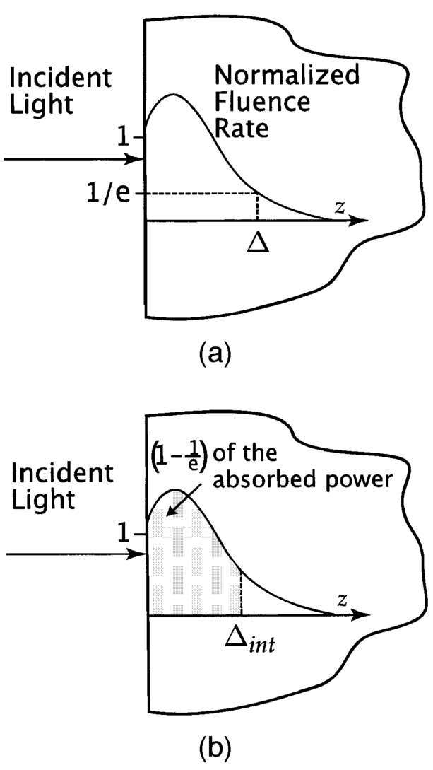
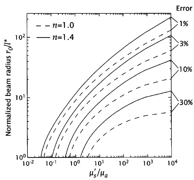
1. Introduction

Many biophotonics applications require knowledge of the light distribution produced by illumination of a turbid tissue with a collimated laser beam.¹ Examples include photodynamic therapy, photon migration spectroscopy, and optoacoustic imaging. If one considers light propagating as a neutral particle, the Boltzmann transport equation provides an exact description of radiative transport.² However, the Boltzmann transport equation is an integrodifferential equation that often cannot be solved analytically. As an alternative, investigators have resorted to a variety of analytic and computational methods, including Monte Carlo simulations, the adding-doubling method, and functional expansion methods.² ³ ⁴ ⁵ ⁶ Each of these methods possesses unique limitations. For example, while Monte Carlo simulations provide solutions to the Boltzmann transport equation that are exact within statistical uncertainty, they require significant computational resources.⁷ ⁸ ⁹ While, numerical finite difference or finite element solutions for the Boltzmann transport equation¹⁰ may involve less computational expenditure, they require spatial and angular discretizations of the computational domain that lead to inaccuracies that are often difficult to quantify. Finally functional expansion methods, such as the standard diffusion approximation (SDA), that express the angular distribution of the light field and the single-scattering-phase function as a truncated series of spherical harmonics are typically accurate only under a limiting set of conditions.² ⁶ ¹¹ ¹² ¹³

Although the SDA provides only an approximate solution to the Boltzmann transport equation, its computational simplicity has proven valuable for applications in optical diagnostics and therapeutics. Unfortunately, the limitations of the SDA are significant and confine its applicability to highly scattering media and to locations distal from both collimated sources and interfaces possessing significant mismatches in refractive index.¹¹ ¹⁴ ¹⁵ ¹⁶ Such conditions are not satisfied in many biomedical laser applications and, over the past 15 yr, hybrid Monte Carlo–diffusion methods¹⁷ ¹⁸ as well as the δ-P₁, P₃, and δ-P₃ approximations have been proposed as improved radiative transport models.¹ ⁶ ¹⁹ ²⁰ ²¹ ²² ²³ ²⁴ ²⁵ Our focus here is the δ-P₁ (or δ-Eddington) model first introduced in 1976 by Joseph et al.;²⁶ and first applied to problems in the biomedical arena independently by Prahl,²³ ²⁷ by Star,⁶ ²⁴ and Star et al.;²⁵

Many investigators in biomedical optics have studied the accuracy of functional expansion methods. Groenhuis et al.; provided one of the first comparative studies between Monte Carlo and SDA predictions for the spatially resolved diffuse reflectance produced by illumination of a turbid medium with a finite diameter laser beam.¹¹ Later, Flock et al.; provided another comparison between Monte Carlo simulations and the SDA that focused primarily on optical dosimetry; specifically the accuracy of fluence rate profiles and optical penetration depth predictions for planar irradiation of a turbid medium.²⁸ More recently, Venugopalan et al.; presented analytic solutions for radiative transport within the δ-P₁ approximation for infinite media illuminated with a finite spherical source.¹⁹ The accuracy of these solutions was demonstrated by comparison with experimental measurements made in phantoms over a broad range of optical properties. Spott and Svaasand reviewed a number of formulations of the diffusion approximation (P₁, δ-P₁, δ-P₃) for a semi-infinite medium illuminated with a collimated light source, and compared fluence rate and diffuse reflectance predictions with Monte Carlo simulations for optical properties representative of in vivo conditions.¹⁶ Dickey et al.;²⁰ ²¹ as well as Hull and Foster²² have studied the improvements in accuracy offered by the P₃ approximation for predicting both fluence rate profiles and spatially resolved diffuse reflectance. These studies have confirmed that the δ-P₁ approach can provide significant improvements in radiative transport predictions relative to SDA with minimal additional complexity.

While these investigations have provided some indication of the improved accuracy provided by the δ-P₁ approximation relative to the SDA, none have offered a quantitative assessment of its performance against a radiative transport benchmark such as Monte Carlo simulations over a wide range of optical properties. Thus, it is difficult to establish a priori the loss of accuracy that one suffers when using the δ-P₁ approximation to determine fluence rate distributions or optical penetration depths. Our objective is to provide a comprehensive quantitative assessment of the accuracy of optical dosimetry predictions provided by the δ-P₁ approximation when a turbid semi-infinite medium is exposed to collimated radiation. Here, we report on the variation of the δ-P₁ model accuracy with tissue optical properties and diameter of the incident laser beam.

Specifically, we determined the fluence rate profiles predicted by the δ-P₁ approximation for semi-infinite media when subjected to planar (1-D) or Gaussian beam (2-D) irradiation. For comparison, we performed Monte Carlo simulations to provide “benchmark” solutions of the Boltzmann transport equation for multiple sets of optical properties. While we include plots of diffuse reflectance R_d versus (μ_s ^′/μ_a) for planar irradiation, our focus is on the internal light distribution as represented by the spatial variation of the fluence rate. Since it is cumbersome to display the variation of fluence rate with depth for more than a few sets of optical properties, we also examined predictions for the optical penetration depth. Comparison of the optical penetration depths predicted by the δ-P₁ approximation with those derived from Monte Carlo simulations enables a continuous assessment of the δ-P₁ model accuracy over a broad range of optical properties. These results are presented within a dimensionless framework to enable rapid estimation of the light distribution in a medium of known optical properties. Moreover, to provide quantitative error assessment, we include plots of the difference between the δ-P₁ and Monte Carlo estimates. The variation of these errors with tissue optical properties and irradiation conditions provide much insight into the nature and origin of the deficiencies inherent in the δ-P₁ approximation as well as other functional expansion methods.

2. δ-P ₁ Model Formulation and Monte Carlo Computation

2.1.

δ-P₁ Approximation of the Single-Scattering Phase Function

The basis of the δ-P₁ approximation to radiative transport is the δ-P₁ phase function as formulated by Joseph et al.;²⁶

Eq. (1)

p_{δ} - P_{1} (\hat{ω} \cdot {\hat{ω}}^{'}) = \frac{1}{4 π} {2 f δ [1 - (\hat{ω} \cdot {\hat{ω}}^{'})] + (1 - f) [1 + 3 g^{*} (\hat{ω} \cdot {\hat{ω}}^{'})]},

where ω^ and ω^^′ are unit vectors that represent the direction of light propagation before and after scattering, respectively. In Eq. (1) f is the fraction of light scattered directly forward, which the δ-P₁ model treats as unscattered light. The remainder of the light (1−f ) is diffusely scattered according to a standard P₁ (or Eddington) phase function with single scattering asymmetry g^*. To determine appropriate values for f and g^*, one must choose a phase function to approximate. In this paper, we choose to provide results for the Henyey-Greenstein phase function, as it is known to provide a reasonable approximation for the optical scattering in biological tissues²⁹:

Eq. (2)

p_{H G} (\hat{ω} \cdot {\hat{ω}}^{'}) = \frac{1}{4 π} \frac{1 - g_{1}^{2}}{{[1 - 2 g_{1} (\hat{ω} \cdot {\hat{ω}}^{'}) + g_{1}^{2}]}^{3 / 2}}

Recalling that for a spatially isotropic medium, the n^th moment, g_n, of the phase function p(ω^⋅ω^^′) is defined by

Eq. (3)

g_{n} = 2 π \int_{- 1}^{1} P_{n} (\hat{ω} \cdot {\hat{ω}}^{'}) p (\hat{ω} \cdot {\hat{ω}}^{'}) d (\hat{ω} \cdot {\hat{ω}}^{'}),

where P_n is the n^th Legendre polynomial, we determine f and g^* by requiring the first two moments of the δ-P₁ phase function, g₁=f+(1−f )g^* and g₂=f, to match the corresponding moments of the Henyey-Greenstein phase function, which are given by g_n=g₁ ⁿ. This yields the following expressions for f and g^*:

Eq. (4)

f = g_{1}^{2} a n d g^{*} = g_{1} / (g_{1} + 1) .

For simplicity, from this point forward we refer to g₁ simply as g and all δ-P₁ model results in this paper are shown for g=0.9 unless noted otherwise.

2.2.

δ-P₁ Approximation of the Radiance

In a manner similar to the phase function, the radiance is also separated into collimated and diffuse components:

Eq. (5)

L (r, \hat{ω}) = L_{c} (r, \hat{ω}) + L_{d} (r, \hat{ω}),

where r is the position vector and ω^ is a unit vector representing the direction of light propagation.

For irradiation with a collimated laser beam normally incident on the surface of a semi-infinite medium, the collimated radiance takes the form

Eq. (6)

L_{c} (r, \hat{ω}) = \frac{1}{2 π} E (r, \hat{z}) δ (1 - \hat{ω} \cdot \hat{z}),

where z^ is the direction of the collimated light within the medium, and E(r,z^) is the complete spatial distribution of collimated light provided by the source. While the lateral spatial variation of E(r,z^) is given by the irradiance distribution of the incident laser beam E₀(x,y), its decay with depth (z -dir) is governed by absorption and scattering within the medium. Specifically, loss of collimated light arises from both absorption and diffuse scattering. Noting that in the δ-P₁ phase function only (1−f ) of the incident light is diffusely scattered, the decay of the collimated light with depth will behave as a modified Beer-Lambert law:

Eq. (7)

E (r, \hat{z}) = E_{0} (x, y) (1 - R_{s}) \exp {- [μ_{a} + μ_{s} (1 - f)] z} = E_{0} (x, y) (1 - R_{s}) \exp [- (μ_{a} + μ_{s}^{*}) z],

where R_s is the specular reflectance for unpolarized light, μ_a is the absorption coefficient, μ_s is the scattering coefficient, and μ_s ^*≡μ_s(1−f ) is a reduced scattering coefficient. For a collimated beam traveling along the z axis that possesses either a uniform or Gaussian irradiance profile we can work in cylindrical (r,z) rather than Cartesian (x,y,z) coordinates. In this case, the collimated fluence rate is given by

Eq. (8)

φ_{c} (r) = \int_{4 π} L_{c} (r, \hat{ω}) = E (r, \hat{z}) = E_{0} (r) (1 - R_{s}) \exp (- μ_{t}^{*} z),

where E₀(r) is the radial irradiance distribution of the incident laser beam and μ_t ^*≡μ_a+μ_s ^*.

The diffuse radiance in Eq. (5) is approximated, as in the SDA, by the sum of the first two terms in a Legendre polynomial series expansion:

Eq. (9)

L_{d} (r, \hat{ω}) = \frac{1}{4 π} \int_{4 π} L_{d} (r, \hat{ω}) d Ω + \frac{3}{4 π} \int_{4 π} L_{d} (r, {\hat{ω}}^{'}) ({\hat{ω}}^{'} \cdot {\hat{ω}}^{}) d Ω^{'} = \frac{1}{4 π} φ_{d} (r) + \frac{3}{4 π} j (r) \cdot \hat{ω}

where φ_d(r) is the diffuse fluence rate and j(r) is the radiant flux.

The improved accuracy offered by the δ-P₁ approximation stems from the addition of the Dirac δ function to both the single scattering phase function and the radiance approximation. The δ function provides an additional degree of freedom well suited to accommodate collimated sources and highly forward-scattering media. Thus the addition of the δ function relieves substantially the degree of asymmetry that must be provided by the first-order term in the Legendre expansion.⁶

2.3.

Governing Equations and Boundary Conditions

Substituting Eqs. (1), (6), and (9) into the Boltzmann transport equation and performing balances in both the fluence rate and the radiant flux provides the governing equations in the δ-P₁ approximation for a semi-infinite medium¹⁹:

Eq. (10)

\nabla^{2} φ_{d} (r) - μ_{eff}^{2} φ_{d} (r) = - 3 μ_{s}^{*} μ_{t r} E (r, \hat{z}) + 3 g^{*} μ_{s}^{*} \nabla E (r, \hat{z}) \cdot \hat{z},

Eq. (11)

j (r) = - \frac{1}{3_{μ t r}} [\nabla φ_{d} (r) - 3 g^{*} μ_{s}^{*} E (r, \hat{z}) \hat{z}],

where μ_s ^′≡μ_s(1−g) is the isotropic scattering coefficient, μ_tr≡(μ_a+μ_s ^′) is the transport coefficient, and μ_eff≡(3μ_aμ_tr)^1/2 is the effective attenuation coefficient.

Two boundary conditions are required to solve Eqs. (10) and (11). At the free surface of the medium, we require conservation of the diffuse flux component normal to the interface, which yields

Eq. (12)

[φ_{d} (r) - A h \nabla φ_{d} (r) \cdot \hat{z}] |_{z = 0} = - 3 A h g^{*} μ_{s}^{*} E (r, \hat{z}) |_{z = 0},

where A=(1+R₂)/(1−R₁) and h=2/3μ_tr. Here R₁ and R₂ are the first and second moments of the Fresnel reflection coefficient for unpolarized light and are given by

Eq. (13)

R_{1} = 2 \int_{0}^{1} r_{F} (ν) ν d ν and R_{2} = 3 \int_{0}^{1} r_{F} (ν) ν^{2} d ν,

where ν=ω^⋅z^, with z^ defined as the inward pointing unit vector normal to the surface. The details of this derivation are provided in Appendix A. Note that Eq. (12) represents an exact formulation for conservation of energy at the boundary and avoids the approximations inherent in the use of extrapolated boundary conditions.³⁰ ³¹ The second boundary condition requires the diffuse light field to vanish in regions far away from the source. Thus,

Eq. (14)

φ_{d} (r) |_{r \to \infty} \to 0.

2.4.

Solutions for Planar and Gaussian Beam Irradiation

The total fluence rate is given by the sum of the collimated and diffuse fluence rates:

Eq. (15)

φ (r) = φ_{c} (r) + φ_{d} (r) .

2.4.1.

Collimated fluence rate

For either planar or Gaussian beam irradiation conditions, as shown in Fig. 1, the collimated fluence rate within the tissue is expressed in the form

Eq. (16)

φ_{c} (r, z) = E_{0} (r) (1 - R_{s}) \exp (- μ_{t}^{*} z) .

For planar irradiation, E₀(r)=E₀ while for Gaussian beam irradiation, E₀(r)=E₀ exp(−2r²/r₀ ²), where r₀ is the Gaussian beam radius, i.e., the radial location where the irradiance falls is 1/e² of the maximum irradiance. Note that E₀=2P/πr₀ ², where E₀ denotes the peak irradiance and P is the incident power of the Gaussian laser beam. For generality, we define a normalized collimated fluence rate φ¯_c as

Eq. (17)

{\bar{φ}}_{c} = \frac{φ_{c} (r, z)}{E_{0} (r) (1 - R_{s})} = \exp (- μ_{t}^{*} z) .

Figure 1

Depiction of (a) planar and (b) Gaussian beam irradiation conditions.

2.4.2.

Diffuse fluence rate for planar irradiation

For planar illumination the diffuse fluence rate is determined by solving Eq. (10) subject to the boundary conditions Eqs. (12) and (14) and yields

Eq. (18)

φ_{d} (z) = E_{0} (1 - R_{s}) [α \exp (- μ_{t}^{*} z) + β \exp (- μ_{e f f^{z}})],

where

Eq. (19)

α = \frac{3 μ_{s}^{*} (μ_{t}^{*} + g^{*} μ_{a})}{μ_{eff}^{2} - μ_{t}^{* 2},}

and

Eq. (20)

β = \frac{- α (1 + A h μ_{t}^{*}) - 3 A h g^{*} μ_{s}^{*}}{(1 + A h μ_{eff})} .

The solution procedure is detailed in Appendix B. In a manner analogous to the collimated fluence rate, we define a normalized diffuse fluence rate φ¯_d as

Eq. (21)

{\bar{φ}}_{d} (z) = \frac{φ_{d} (z)}{E_{0} (1 - R_{s})} = α \exp (- μ_{t}^{*} z) + β \exp (- μ_{e f f^{z}}) .

2.4.3.

Diffuse fluence rate for Gaussian beam irradiation

For Gaussian beam irradiation, the diffuse fluence rate is given by

Eq. (22)

φ_{d} (r, z) = E_{0} (1 - R_{s}) \int_{0}^{\infty} {γ \exp (- μ_{t}^{*} z) + ξ \exp [- {(k^{2} + μ_{eff}^{2})}^{1 / 2} z]} J_{0} (k r) k d k,

where

Eq. (23)

γ = \frac{3 μ_{s}^{*} (μ_{t}^{*} + g^{*} μ_{a}) r_{0}^{2} \exp (- r_{0}^{2} k^{2} / 8)}{4 (k^{2} + μ_{eff}^{2} - μ_{t}^{* 2})},

Eq. (24)

ξ = \frac{- 3 g^{*} μ_{s}^{*} r_{0}^{2} \exp (- r_{0}^{2} k^{2} / 8) - 4 γ [{(A h)}^{- 1} + μ_{t}^{*}]}{4 [{(A h)}^{- 1} + {(k^{2} + μ_{eff}^{2})}^{1 / 2}]},

and J ₀ is the zeroth-order Bessel function of the first kind. The solution procedure is detailed in Appendix C. The normalized fluence rate for Gaussian beam irradiation is given by

Eq. (25)

{\bar{φ}}_{d} (r, z) = \int_{0}^{\infty} {γ \exp (- μ_{t}^{*} z) + ξ \exp [- {(k^{2} + μ_{eff}^{2})}^{1 / 2} z]} J_{0} (k r) k d k .

Numerical methods (MATLAB, MathWorks, Natick, Massachusetts) were employed to compute the definite integral in Eqs. (22) and (25).

2.5.

Diffuse Reflectance for Planar Irradiation

The prediction of the diffuse reflectance provided by the δ-P₁ approximation is

Eq. (26)

R_{d} = {\frac{- j (z) \cdot \hat{z}}{E_{0} (1 - R_{s})} |}_{z = 0} = \frac{1}{3 μ t r E_{0} (1 - R_{s})} {[3 g^{*} μ_{s}^{*} E_{0} \exp (- μ_{t}^{*} z) - \frac{d φ_{d} (z)}{d z}] |}_{z = 0} = {\frac{{\bar{φ}}_{d} (z)}{2 A} |}_{z = 0} .

2.6.

Limiting Cases

A unique feature of the solutions provided by the δ-P₁ approximation is that φ_d→0 in the limit of vanishing scattering, i.e., when μ_s ^′≪μ_a. Thus in a medium where absorption is dominant μ_t ^*→μ_a and the total fluence rate is governed solely by the collimated contribution, i.e.,

Eq. (27)

\lim_{(μ_{s}^{'} / μ_{a}) \to 0} φ (r, z) = φ_{c} (r, z) = E_{0} (r) (1 - R_{s}) \exp (- μ_{a} z) .

Thus, unlike prevalent implementations of the SDA wherein the collimated light source is replaced by a point source placed at a depth z=(1/μ_s ^′) within the medium, the δ-P₁ approximation correctly recovers Beer’s law in the limit of no scattering.

For media in which scattering is dominant (μ_s ^′≫μ_a or μ_t ^*≫μ_eff), the total fluence rate resulting from planar irradiation reduces to

Eq. (28)

\lim_{(μ_{s}^{'} / μ_{a}) \to \infty} φ (z) = E_{0} (1 - R_{s}) [(3 + 2 A) \exp (- μ_{e f f^{z}}) - 2 \exp (- μ_{t}^{*} z)] .

If we further consider this fluence rate in the far field (large z), Eq. (28) reduces to

Eq. (29)

\lim_{(μ_{s}^{'} / μ_{a}) \to \infty} φ (z) = E_{0} (1 - R_{s}) (3 + 2 A) \exp (- μ_{e f f^{z}}) f o r l a r g e z .

Equation (29) is equivalent to the fluence rate prediction given by the SDA.¹³ Thus, in the limit of high scattering, and away from boundaries and collimated sources, the solution provided by the δ-P₁ approximation properly reduces to that given by the SDA.

2.7.

Optical Penetration Depth

Apart from the fluence rate profiles and diffuse reflectance results offered by the δ-P₁ approximation, we are also interested in its predictions for the characteristic optical penetration depth (OPD) in the tissue. In Fig. 2, we display two variations of the OPD that we consider in this study. The first penetration depth metric Δ is simply the depth at which the fluence rate falls to 1/e of the incident fluence rate after accounting for losses due to specular reflection. The second penetration depth metric Δ_int is the depth at which all but 1/e of the power of the laser radiation has been absorbed after accounting for losses due to both specular and diffuse reflection. For generality, we normalize both these metrics relative to a characteristic length scale. We choose (1/μ_eff) for this length scale as it is the traditional definition for the optical penetration depth³² and is the length scale over which the homogenous solution to Eq. (10) decays. Accordingly we define

Eq. (30)

\bar{Δ} \equiv μ_{eff} Δ and \bar{Δ} i n t \equiv μ_{eff} Δ i n t .

Figure 2

Graphical depiction of optical penetration depths (a) Δ and (b) Δ_int.

2.8.

Monte Carlo Simulations

We performed Monte Carlo simulations for planar and Gaussian beam irradiation of semi-infinite media under both refractive index matched and mismatched conditions. For this purpose we employed code derived from the Monte Carlo Multi-Layer (MCML) package written by Wang et al.;⁸ ⁹ that computes the 3-D fluence rate distribution and spatially resolved diffuse reflectance corresponding to irradiation with a laser beam possessing either uniform or Gaussian profiles. A Henyey-Greenstein phase function was utilized with a single scattering asymmetry coefficient of g=0.9 unless stated otherwise. This value of g was chosen as it is representative of many biological tissues.²⁹ To approximate planar irradiation conditions we used a beam with a uniform irradiance profile with radius r₀=200l^*, where l^*≡(1/μ_tr) is the transport mean free path. For Gaussian beam illumination, we set r₀ to the desired 1/e² radius of the laser beam. To provide sufficient spatial resolution a minimum of 100 grid points were contained within one beam radius. Between 10⁷ and 2×10⁹ photons were launched for each simulation and resulted in fluence rate estimates with relative standard deviation of less than 0.1.

3. Results and Discussion

3.1.

Planar Illumination

Figures 3(a) and 3(b) provide normalized fluence rate profiles predicted by the δ-P₁ approximation and Monte Carlo simulations under planar illumination conditions for 0.3⩽(μ_s ^′/μ_a)⩽100 and relative refractive indices n=(n₂/n₁)=1.0 and 1.4, respectively. Note that the profiles are plotted against a reduced depth that is normalized relative to the transport mean free path l^*. These figures also provide the error of the δ-P₁ predictions relative to the Monte Carlo estimates.

Figure 3

Normalized fluence rate φ¯ versus reduced depth (z/l^*) as predicted by the δ-P₁ approximation (solid curves) and Monte Carlo simulations (symbols) for planar illumination under refractive index (a) matched (n=1.0) and (b) mismatched (n=1.4) conditions. Profiles are shown for (μ_s ^′/μ_a)=100 (○), 10 (*), 3 (⋄), 1 (×), and 0.3 (•) with g=0.9. Lower plots show the percentage error of the δ-P₁ predictions relative to the Monte Carlo simulations using the same symbols as the main plot.

Overall, the performance of the δ-P₁ approximation is impressive. The fluence rate is predicted with an error of ⩽12 over the full range of optical properties. In the far field, the model performance is exceptional for large (μ_s ^′/μ_a), degrades slightly when scattering is comparable to absorption (μ_s ^′≃μ_a), and improves again when absorption dominates scattering (μ_s ^′/μ_a≲0.3). This behavior is expected. For large (μ_s ^′/μ_a) the prevalence of multiple scattering enables the diffuse component of the δ-P₁ approximation to provide an accurate description of the light field. However, when scattering is still significant but (μ_s ^′/μ_a) is reduced, the decay of the light field occurs on a spatial scale intermediate to that predicted by diffusion, i.e., exp(−μ_effz), and that predicted by the total interaction coefficient, i.e., exp(−μ_t ^*z). This results in an error between the δ-P₁ model and the Monte Carlo estimates that increases with increasing depth. This is seen most notably for the case of (μ_s ^′/μ_a)=1 for which the error is largest in the far field. Finally, for highly absorbing media, the overall accuracy of the δ-P₁ approximation improves again because the contribution of collimated irradiance to the total light field increases markedly and is well described by the modified Beer-Lambert law of Eq. (7).

In the near field, the accuracy of the δ-P₁ approximation degrades with increasing (μ_s ^′/μ_a). The origin of this lies in the fact that increases in scattering result in increased amounts of light backscattered toward the surface. This leads to an increase in the angular asymmetry in the diffuse component of the light field near the surface which is not accurately modeled by a radiance approximation that simply employs a constant and the first-order Legendre polynomial. The δ-P₁ model performs worse for n=1.4 because the refractive index mismatch introduces internal reflection that further enhances the angular asymmetry of the light field near the surface. However, when scattering is less prominent, the accuracy of the fluence rate profiles is not as strongly dependent on the refractive index mismatch because there is less light backscattered toward the surface.

We also examined the influence of the single scattering asymmetry coefficient g on the δ-P₁ model predictions for fixed values of (μ_s ^′/μ_a). Figures 4(a) and 4(b) show the variation of the normalized fluence rate profiles for 0⩽g⩽0.9 and (μ_s ^′/μ_a)=100 for n=1 and 1.4, respectively. Figures 5(a) and 5(b) show these same results in media with (μ_s ^′/μ_a)=1. In the highly scattering case, the effect of g is seen most prominently in the near field due to its impact on the boundary condition used in the δ-P₁ approximation. However, the effect is small and results in changes of the error between δ-P₁ and Monte Carlo (MC) estimates that do not exceed 4 relative to results found for g=0.9. Note that for (μ_s ^′/μ_a)=100, the value of g does not affect the predictions in the far field as the SDA limit is applicable. As a result the decay of the fluence rate profiles is governed by exp(−μ_effz) and is independent of g for a fixed (μ_s ^′/μ_a). By contrast, for (μ_s ^′/μ_a)=1, the variation in g affects the errors most prominently in the far field. This occurs because there is minimal backscattering due to the higher absorption in the medium leading to a fluence rate profile whose decay is dependent on g even for a fixed (μ_s ^′/μ_a). However, we again see that the effect of g is minimal as the variations in the error are less than 7 even in the far field. Given that these error variations are small and the fact that most soft biological tissues are strongly forward scattering we show all remaining results for a value of g=0.9 (Ref. 29).

Figure 4

Normalized fluence rate φ¯ versus reduced depth (z/l^*) as predicted by the δ-P₁ approximation (solid curves) and Monte Carlo simulations (symbols) for planar illumination under refractive index (a) matched (n=1.0) and (b) mismatched (n=1.4) conditions. Profiles are shown for g=0 (○), 0.3 (*), 0.7 (×), and 0.9 (•) with (μ_s ^′/μ_a)=100. Lower plots show the percentage error of the δ-P₁ predictions relative to the Monte Carlo simulations using the same symbols as the main plot.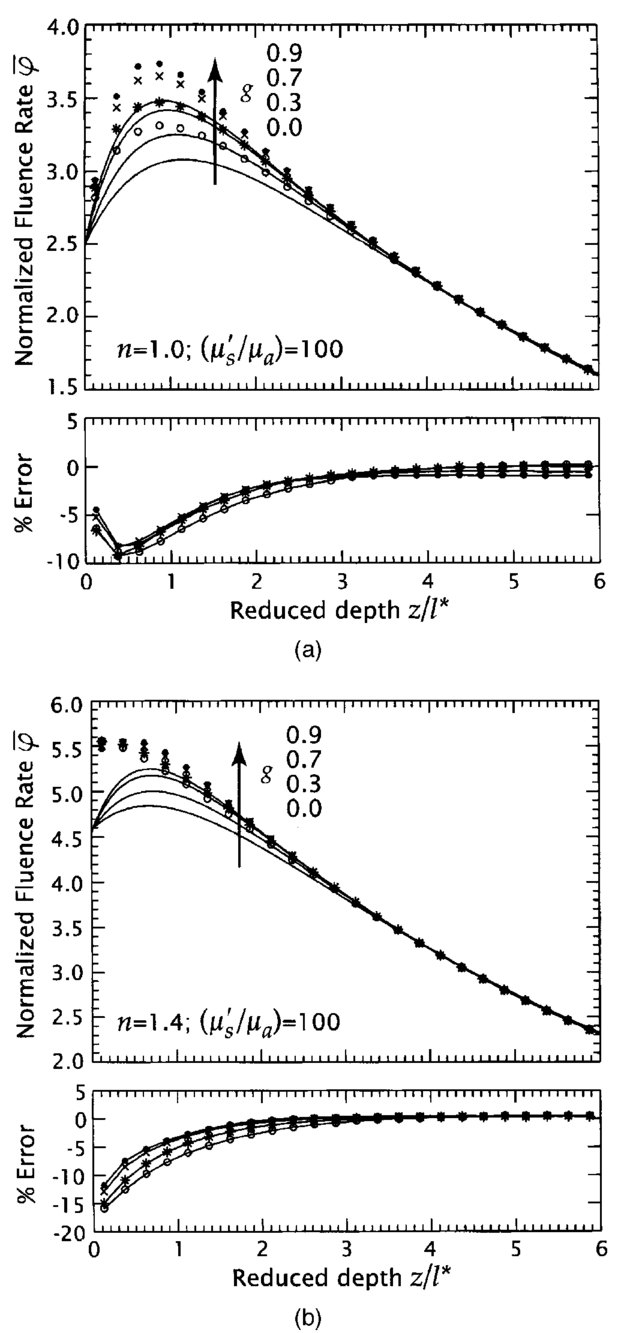

Figure 5

Normalized fluence rate φ¯ versus reduced depth (z/l^*) as predicted by the δ-P₁ approximation (solid curves) and Monte Carlo simulations (symbols) for planar illumination under refractive index (a) matched (n=1.0) and (b) mismatched (n=1.4) conditions. Profiles are shown for g=0 (○), 0.3 (*), 0.7 (×), and 0.9 (•) with (μ_s ^′/μ_a)=1. Lower plots show the percentage error of the δ-P₁ predictions relative to the Monte Carlo simulations using the same symbols as the main plot.

Figures 6(a) and 6(b) present the variation of the diffuse reflectance R_d with (μ_s ^′/μ_a) for n=1.0 and 1.4, respectively. As in Fig. 3, there is good agreement for large (μ_s ^′/μ_a) independent of the refractive index mismatch. Under index-matched conditions, there is no internal reflection at the surface and R_d is predicted with a relative error of ±8. For a refractive index mismatch corresponding to a tissue-air interface, the model predictions degrade as (μ_s ^′/μ_a) is reduced. Specifically, relative errors exceed 15 for (μ_s ^′/μ_a)<3. However, as (μ_s ^′/μ_a)→0 the model is bound to recover its accuracy since the diffuse component vanishes and R_d→0 as (μ_s ^′/μ_a)→0. Moreover, for (μ_s ^′/μ_a)<0.3 the amount of diffuse reflectance is negligible for all practical purposes. Thus while the relative error in R_d may be large, the absolute error is vanishingly small.

Figure 6

Diffuse reflectance R_d versus (μ_s ^′/μ_a) as predicted by the δ-P₁ approximation (solid curves) and MC simulations (•) for planar illumination under refractive index (a) matched (n=1.0) and (b) mismatched (n=1.4) conditions. Lower plots show the percentage error of the δ-P₁ predictions relative to the MC simulations.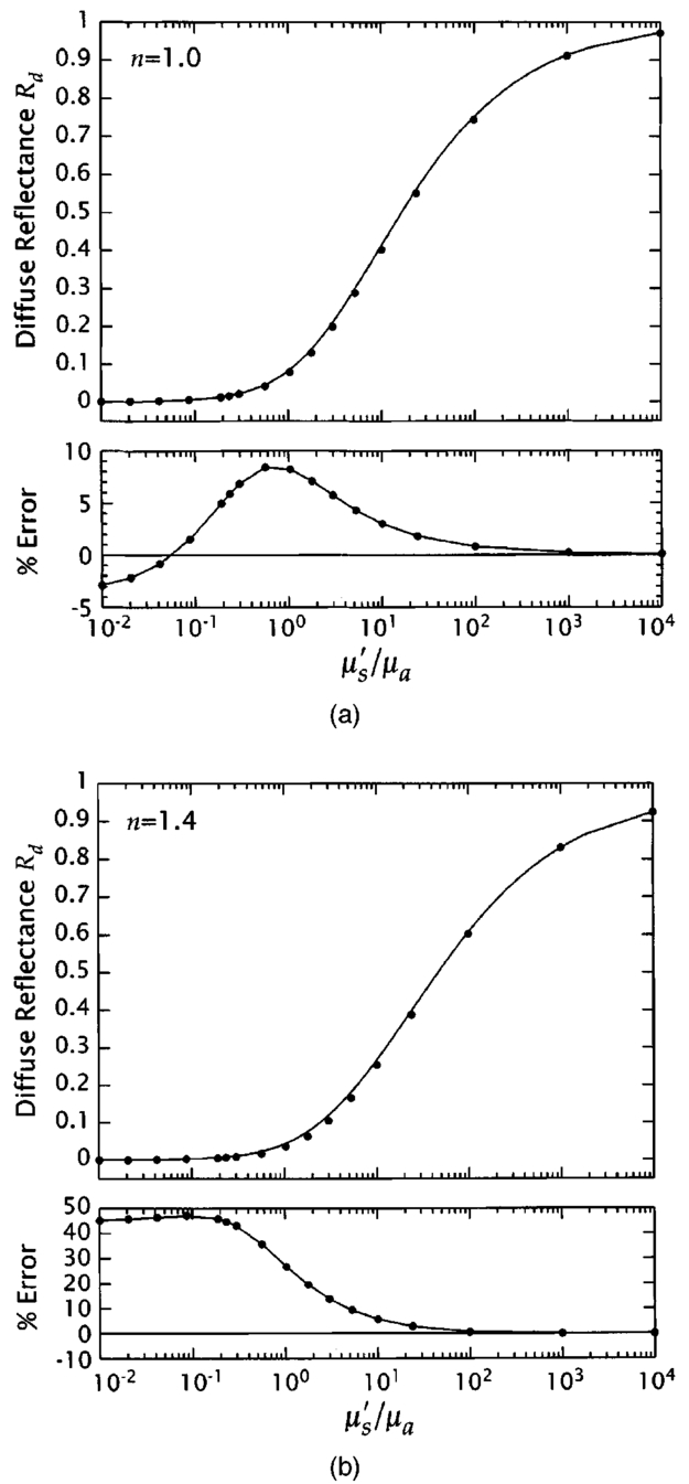

To better characterize the variation in accuracy of the δ-P₁ approximation with (μ_s ^′/μ_a) we examine the OPDs that characterize the fluence rate profiles. Figures 7(a) and 7(b) present estimates for the normalized OPD metrics Δ¯≡μ_effΔ and Δ¯_int≡μ_effΔ_int as predicted by the δ-P₁ approximation and MC predictions for 10⁻²⩽(μ_s ^′/μ_a)⩽10⁴ under refractive index matched (n=1.0) and mismatched (n=1.4) conditions, respectively.

Figure 7

Normalized optical penetration depths Δ¯≡μ_effΔ (○) and Δ¯_int≡μ_effΔ_int (•) versus (μ_s ^′/μ_a) as predicted by the δ-P₁ approximation (solid curves) and MC simulations (symbols) for planar illumination under refractive index (a) matched (n=1.0) and (b) mismatched (n=1.4) conditions. Lower plots show the percentage error of the δ-P₁ predictions relative to the MC simulations.

Note that under conditions of dominant absorption, i.e., (μ_s ^′/μ_a)→0, μ_eff→⊡3μ_a. Thus both Δ¯ and Δ¯_int approach (1/μ_a)(μ_eff)=⊡3 as (μ_s ^′/μ_a)→0. This result is confirmed in Figs. 7(a) and 7(b). In the limit of high scattering, i.e., (μ_s ^′/μ_a)→∞, inspection of Eq. (29) reveals that the value of Δ¯ is dependent on the refractive index mismatch through the boundary parameter A. Setting Eq. (29) equal to E₀(1−R_s)/e and solving we find that Δ¯=1+ln(3+2A). Thus, for (μ_s ^′/μ_a) →∞, the δ-P₁ approximation predicts that Δ¯ →2.61 and 3.19 for n=1.0 and 1.4, respectively. By contrast, a similar analysis reveals that Δ¯_int is not sensitive to the refractive index mismatch and Δ¯_int→1 as (μ_s ^′/μ_a)→∞. These asymptotic limits predicted by the δ-P₁ model are confirmed by the results shown in Figs. 7(a) and 7(b). Overall the δ-P₁ predictions for the optical penetration depth are impressive and match the MC estimates to within ±4 over the entire range of (μ_s ^′/μ_a). The highest relative errors occur at (μ_s ^′/μ_a)≃1 as expected from the characteristics of the fluence rate profiles shown in Fig. 3. Better accuracy is observed for Δ¯ (±2) than for Δ¯_int (±4). This is due to the stronger impact that underestimation of the fluence rate near the surface has on the determination of Δ¯_int.

3.2.

Gaussian Beam Illumination

Figures 8(a) and 8(b) provide normalized fluence rate profiles along the beam centerline (r=0) as predicted by the δ-P₁ approximation and MC simulations at (μ_s ^′/μ_a)=100 for beam radii r₀=100l^*, 30l^*, 10l^*, 3l^*, and 1l^* with n=1.0 and 1.4, respectively. The errors of the δ-P₁ predictions relative to the MC estimates are shown below the main plots. The fluence rate along the beam centerline for r₀=100l^* differs by less than ±0.5 from that produced by planar irradiation. For both n=1.0 and 1.4, the δ-P₁ approximation provides good accuracy relative to the MC predictions for beam radii r₀>3l^* (±17 in the near field, ±5 in the far field). However, the model accuracy degrades for smaller beam radii and reaches ±25 for r₀=l^*. This is expected given that the diffusion model breaks down when length scales comparable to l^* are considered.

Figure 8

Normalized fluence rate along the beam centerline φ¯(r=0) versus reduced depth (z/l^*) as predicted by the δ-P₁ approximation (solid curves) and MC simulations (symbols) for Gaussian beam illumination under refractive index (a) matched (n=1) and (b) mismatched (n=1.4) conditions. Profiles are shown for (μ_s ^′/μ_a)=100 with r₀=100l^* (○), 30l^* (*), 10l^* (⋄), 3l^* (×), 1l^* (•), and g=0.9. Lower plots show the percentage error of the δ-P₁ predictions relative to the MC simulations.

Figures 9(a) and 9(b) provide results for the more challenging case of (μ_s ^′/μ_a)=1. Due to the reduced scattering dispersion that occurs in media of higher absorption, one must consider much smaller beam diameters before the fluence rate profiles along the center differ noticeably from the planar irradiation case. Specifically, for (μ_s ^′/μ_a)=1, the fluence rate along the beam centerline for r₀=30l^* differs by less than ±0.5 from that produced by planar irradiation. For r₀>3l^*, errors in the fluence rate predictions provided by the δ-P₁ model relative to the MC estimates are ±3 in the near field and ±22 in the far field. However, for r₀=l^*, the fluence rate is overestimated by nearly 100 in the far field. While a 100 error may appear striking, one should notice that this occurs once the fluence rate has already dropped by more than two orders of magnitude relative to the surface value. Thus, while the percentage error is large, the error with respect to the overall energy balance is small. This large relative error for small beam radii is not surprising given the great difficulty that low-order functional expansion methods have in modeling the light field when μ_s ^′≃μ_a. In the far field, the accuracy of the δ-P₁ model is nearly independent of the refractive index for the same reasons as those discussed in Sec. 3.1.

Figure 9

Normalized fluence rate along the beam centerline φ¯(r=0) versus reduced depth (z/l^*) as predicted by the δ-P₁ approximation (solid curves) and MC simulations (symbols) for Gaussian beam illumination under refractive index (a) matched (n=1.0) and (b) mismatched (n=1.4) conditions. Profiles are shown for (μ_s ^′/μ_a)=1 with r₀=30l^* (○), 10l^* (⋄), 3l^* (×), 1l^* (•), and g=0.9. Lower plots show the percentage error of the δ-P₁ predictions relative to the MC simulations.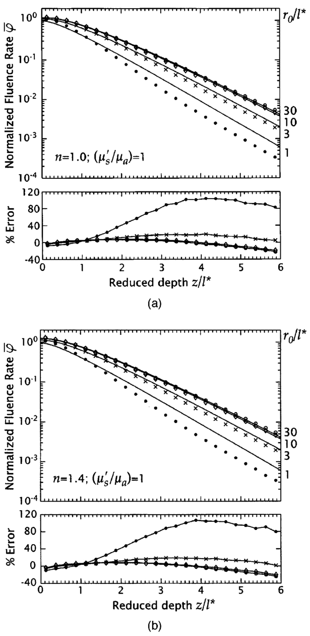

Figures 10(a) and 10(b) provide the normalized OPD Δ¯ along the beam centerline for Gaussian irradiation as predicted by the δ-P₁ model and MC simulations for 10⁻²⩽(μ_s ^′/μ_a)⩽10⁴ and beam radii r₀=1–100l^* with n=1.0 and 1.4, respectively. Corresponding results for Δ¯_int are presented similarly in Figs. 11(a) and 11(b). The OPDs determined in the 1-D case are included for comparison as are the corresponding relative errors. The expected limiting behavior for (μ_s ^′/μ_a)→0 is identical to that in the planar irradiation case and thus both Δ¯ and Δ¯_int converge to ⊡3. For large (μ_s ^′/μ_a) the decay of the fluence rate with depth for finite beam illumination occurs on a spatial scale smaller than exp(−μ_effz) because as the incident laser beam propagates in the medium, optical scattering results in significant lateral dispersion from the high fluence region along the beam centerline to the periphery. Thus Δ¯, Δ¯_int→0 as (μ_s ^′/μ_a)→∞. The δ-P₁ predictions for Δ¯ and Δ¯_int track the MC estimates well, with errors of less than ±4 in Δ¯ and ±20 in Δ¯_int for the smallest beam radius studied (r₀=l^*). Once again, the largest errors occur for μ_s ^′≃μ_a and Δ¯ is predicted more accurately than Δ¯_int. Both of these features are consistent with the fluence rate profiles shown in Figs. 8 and 9 where the largest errors are observed close to the surface (z<2l^*) and for μ_s ^′≃μ_a.

Figure 10

Normalized optical penetration depth Δ¯ versus (μ_s ^′/μ_a) as predicted by the δ-P₁ approximation (solid curves) and MC simulations (symbols) along the beam centerline for Gaussian beam illumination for g=0.9 with r₀=100l^* (○), 30l^* (*), 10l^* (⋄), 3l^* (×), and 1l^* (•) under refractive index (a) matched (n=1.0) and (b) mismatched (n=1.4) conditions. The optical penetration depth for planar illumination predicted by the δ-P₁ approximation is plotted as a dashed curve. Lower plots shows the percentage error of the δ-P₁ predictions relative to the MC simulations.

Figure 11

Normalized optical penetration depth Δ¯_int versus (μ_s ^′/μ_a) as predicted by the δ-P₁ approximation (solid curves) and MC simulations (symbols) along the beam centerline for Gaussian illumination for g=0.9 with r₀=100l^* (○), 30l^* (*), 10l^* (⋄), 3l^* (×), and 1l^* (•) under refractive index (a) matched (n=1.0) and (b) mismatched (n=1.4) conditions. The optical penetration depth for planar illumination predicted by the δ-P₁ approximation is plotted as a dashed line. Lower plots show the percentage error of the δ-P₁ predictions relative to the MC simulations.

Figure 12(a) provides a color contour plot representing the 2-D fluence rate distribution for a Gaussian beam of radius r₀=3l^* with (μ_s ^′/μ_a)=100 and n=1.4. The solid isofluence rate contours and the color map correspond to the prediction provided by the δ-P₁ approximation while the dashed isofluence rate contours represent predictions given by the MC simulations. Figure 12(b) provides the 2-D distribution of the relative errors between the δ-P₁ predictions and the MC simulations. Thus, the δ-P₁ and MC contours shown in Fig. 12(a) provides some indication of the errors in penetration depth that one makes when using the δ-P₁ approximation, while Fig. 12(b) provides the errors in the actual optical dosimetry.

Figure 12

(a) Color contour plot of the normalized fluence rate φ¯(r,z) as predicted by both the δ-P₁ approximation (solid contours and color) and MC simulations (dashed contours) for Gaussian beam irradiation with r₀=3l^* in media with (μ_s ^′/μ_a)=100 for g=0.9 under refractive index mismatched conditions (n=1.4) ; and (b) relative error between δ-P₁ approximation and MC simulations.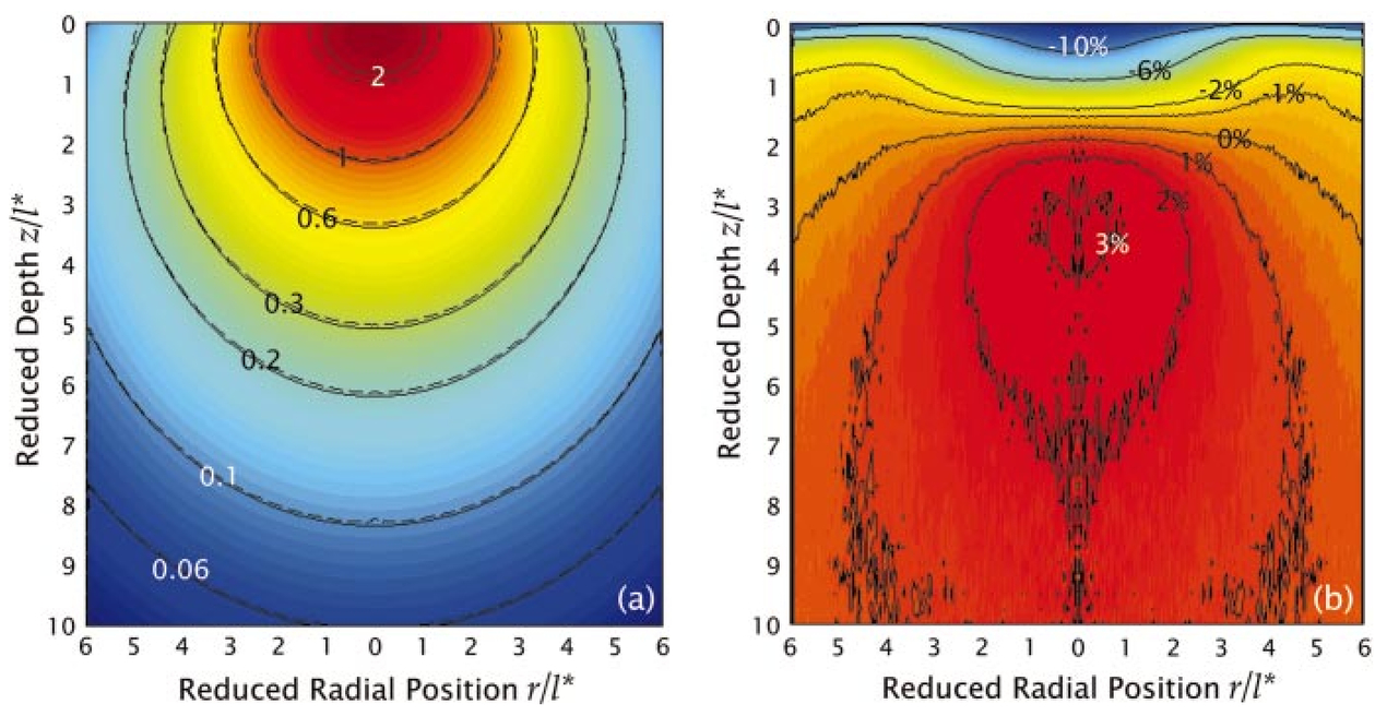

The quality of the δ-P₁ predictions are excellent; the error in the fluence rate relative to the MC estimates never exceeds 20 and is less than 10 over the vast majority of the domain. In the axial direction, the maximum errors occur in the near field close to the boundary, while in the radial direction, they occur along the beam centerline. This is expected because it is at these locations where the spatial gradients and angular asymmetry of the light field are greatest. Figures 13(a) and 13(b) provide plots under identical irradiation conditions for a turbid medium with (μ_s ^′/μ_a)=3. In Fig. 13(a) we see similar errors in the location of the isofluence rate contours when comparing the δ-P₁ approximation relative to the MC predictions. However, in Fig. 13(b), we observe a different spatial pattern and magnitude of the fluence rate errors incurred when using the δ-P₁ approximation rather than a MC estimate. As in Fig. 12(b), the maximum errors in the radial direction occur along the beam centerline. However, in the axial direction, the maximum errors reside in the far field and appear to be increasing with depth. This is similar to the planar irradiation case and occurs because the spatial scale for the decay of the fluence rate with depth lies between exp(−μ_effz) and exp(−μ_t ^*z); thereby leading to poor predictions by the δ-P₁ approximation in the far field under these conditions. It is important to note that examination of δ-P₁ predictions at radial locations away from the centerline reveals equivalent, if not better, accuracy in both fluence rate profiles and OPD metrics. For example, for Gaussian beam radii r₀>3l^*, the errors in both Δ¯ and Δ¯_int at the radial location r=r₀ are ⩽5 and ⩽8, respectively, over the full range of (μ_s ^′/μ_a). This result is consistent with the errors of the full fluence rate distributions shown in Figs. 12 and 13.

Figure 13

(a) Color contour plot of the normalized fluence rate φ¯(r,z) as predicted by both the δ-P₁ approximation (solid contours and color) and MC simulations (dashed contours) for Gaussian beam irradiation with r₀=3l^* in media with (μ_s ^′/μ_a)=3 for g=0.9 under refractive index mismatched conditions (n=1.4) ; and (b) relative error between δ-P₁ approximation and MC simulations.

3.3.

Gaussian Beam versus Planar Irradiation Treatment

As is evident from the results, the use of laser beams of small diameter significantly alters the fluence rate profile and optical penetration depth. For example, Gaussian irradiation of a medium with (μ_s ^′/μ_a)=100 using a beam radius of r₀=3l^* results in a fluence rate that is only ∼50 of that achieved using planar illumination. Moreover, the reduction in both fluence rate and OPD for decreasing beam diameters is more prominent in media with large (μ_s ^′/μ_a) because the scattering enhances lateral dispersion of the collimated radiation (Figs. 8 9 10 11 12 13). However, the Gaussian beam expressions are a bit more formidable than those for the case of planar irradiation. As a result, for simplicity and convenience, it may be useful to determine the conditions under which the results of a planar irradiation analysis provides sufficiently accurate predictions along the centerline of a Gaussian beam. This may obviate the need to use the more complex expressions corresponding to Gaussian beam irradiation in some cases.

Figure 14 provides these results in the form of a contour plot showing the percentage difference between the fluence rate predictions given by the δ-P₁ approximation for Gaussian beam irradiation along the centerline compared to planar irradiation as a function of both normalized beam radius (r₀/l^*) and optical properties (μ_s ^′/μ_a). Contours are provided for differences of 1, 3, 10, and 30 for n=1.0 (solid contours) and 1.4 (dashed contours), respectively. These results indicate that as absorption becomes more dominant, the centerline fluence rate profiles produced by laser beams of smaller diameter can be adequately approximated using the planar irradiation predictions. This can also be seen in the OPD results shown earlier in Figs. 10 and 11. In these figures, we observed that for a given beam radius, there is a certain value of (μ_s ^′/μ_a) above which the OPDs corresponding to Gaussian irradiation drop below the OPDs for planar irradiation. We note that this value of (μ_s ^′/μ_a) becomes lower as smaller beam diameters are used. Note also that the inaccuracies incurred in using the planar irradiation results are always lower for the index-matched case. This is because the presence of a refractive index mismatch results in internal reflection at the tissue-air interface that enhances lateral dispersion of the light field. This additional source of dispersion hastens the need for the use of a radiative transport model that is geometrically faithful to the irradiation conditions.

Figure 14

Contours for the error incurred in predicting fluence rate profiles along the centerline of a Gaussian laser beam of normalized radius r₀/l^* as a function of (μ_s ^′/μ_a) when using δ-P₁ predictions for the planar irradiation case for n=1.0 (dashed) and n=1.4 (solid).

4. Conclusion

We have shown that the δ-P₁ approximation to the Boltzmann transport equation provides remarkably accurate predictions of light distribution and energy deposition in homogeneous turbid semi-infinite media. Examination of the functional expressions involved in the δ-P₁ approximation reveals proper asymptotic behavior in the limits of absorption- and scattering-dominant media. Comparison of the fluence rate and optical penetration depth predictions given by the δ-P₁ approximation with MC simulations demonstrate the greater fidelity and accuracy of the δ-P₁ model relative to the standard diffusion approximation.

The availability of an analytic light transport model providing accurate optical dosimetry predictions is an invaluable tool for the biomedical optics community. By providing our results in terms of dimensionless quantities, they can be used to rapidly estimate the fluence rate distributions and optical penetration depths generated by a wide range of irradiation conditions and tissue optical properties. Thus beyond a greater theoretical understanding of the significant gains to be realized through the use of the δ-P₁ approximation over the standard diffusion approximation, these figures provide the biomedical optics community with charts that can be used for rapid lookup and estimation of light-transport related quantities.

5. Appendix A Derivation of Surface Boundary Conditions in the δ-P ₁ Approximation

The governing equations of the δ-P₁ approximation are (see Sec. 2):

Eq. (31)

\nabla^{2} φ_{d} (r) - 3 μ_{a} μ_{t r} φ_{d} (r) = - 3 μ_{s}^{*} μ_{t r} E (r, \hat{z}) + 3 g^{*} μ_{s}^{*} \nabla E (r, \hat{z}) \cdot \hat{z}

Eq. (32)

j (r) = - \frac{1}{3 μ_{t r}} [\nabla φ_{d} (r) - 3 g^{*} μ_{s}^{*} E (r, \hat{z}) \hat{z}],

where r is the position in the medium, z^ is the unit vector colinear with the direction of the collimated source, E(r,z^) is the irradiance distribution of the collimated source, μ_a is the absorption coefficient, μ_tr≡μ_a+μ_s ^′ is the transport coefficient with μ_s ^′ being the isotropic scattering coefficient, g^* is the single scattering asymmetry coefficient of the P₁ portion of the δ-P₁ phase function, and μ_s ^*≡μ_s(1−f ) is a reduced scattering coefficient. Selection of f and g^* depends on the selection of the phase function as described in Sec. 2.1.

Two boundary conditions are required to solve Eq. (31). Requiring conservation of the diffuse flux component normal to the interface, we obtain⁶ ²³

Eq. (33)

\int_{\hat{ω} \cdot \hat{z} \geq 0} L_{d} (r, \hat{ω}) (\hat{ω} \cdot \hat{z}) d \hat{ω} = \int_{\hat{ω} \cdot \hat{z} < 0} L_{d} (r, \hat{ω}) r_{F} (- \hat{ω} \cdot \hat{z}) (- \hat{ω} \cdot \hat{z}) d \hat{ω},

where z^ is the inward-pointing surface normal, and r_F(−ω^⋅z^) is the Fresnel reflection coefficient for unpolarized light. The preceding condition can be described in words as equating the amount of diffuse light that travels upward (ω^⋅z^<0) and gets internally reflected at the interface with the amount of diffuse light traveling downward (ω^⋅z^⩾0) from the interface.

Substituting the approximation for the diffuse fluence rate given by Eq. (9) and using Eq. (32) to eliminate j(r), we obtain the following form for the surface boundary condition in the δ-P₁ approximation:

Eq. (34)

[φ_{d} (r) - A h \nabla φ_{d} (r) \cdot \hat{z}] |_{z = 0} = - 3 A h g^{*} μ_{s}^{*} E (r, \hat{z}) |_{z = 0},

where A=(1+R₂)/(1−R₁) and h=2/3μ_tr. This result is identical to that provided by Eq. (12). Here R₁ and R₂ are the first and second moments of the Fresnel reflection coefficient for unpolarized light, as given by Eq. (13).

Note that in many implementations of the SDA, A is approximated instead by A≈(1+R₁)/(1−R₁). While this is strictly incorrect, it results in slightly better approximations of the fluence rate in the near field at the expense of providing worse fluence rate approximations in the far field as well as violating conservation of energy when integrating the light field over the entire volume. The following cubic polynomial provides an estimate for A=(1+R₂)/(1−R₁) that typically differs from the exact value by less than 1:²³

Eq. (35)

A (n) = - 0.13755 n^{3} + 4.3390 n^{2} - 4.90366 n + 1.6896.

6. Appendix B Solution of the δ-P ₁ Approximation for Planar Illumination of a Semi-Infinite Medium

For planar illumination the source term is given by

Eq. (36)

E (z, \hat{ω}) = E_{0} (1 - R_{s}) \exp (- μ_{t}^{*} z) δ (1 - \hat{ω} \cdot \hat{z}),

where E₀ is the irradiance, ω^ is the unit direction vector, and z^ is the inward pointing unit vector normal to the surface of the medium and is colinear with the z coordinate axis. Substituting Eq. (36) into Eq. (10), we obtain the governing equation for a planar geometry:

Eq. (37)

\frac{d^{2} φ_{d} (z)}{d z^{2}} - 3 μ_{a} μ_{t r} φ_{d} (z) = - 3 μ_{s}^{*} (μ_{t}^{*} + g^{*} μ_{a}) E_{0} (1 - R_{s}) \exp (- μ_{t}^{*} z) .

The boundary conditions for the 1-D case reduce to

Eq. (38)

{φ_{d} - A h \frac{d φ_{d} (z)}{d z} |}_{z = 0} = - 3 A h g^{*} μ_{s}^{*} E_{0} (1 - R_{s}),

Eq. (39)

φ_{d} (z) |_{z \to \infty} \to 0.

The solution to Eq. (37) satisfying the Eqs. (38) and (39) is

Eq. (40)

φ_{d} (z) = E_{0} (1 - R_{s}) [α \exp (- μ_{t}^{*} z) + β \exp (- μ_{e f f^{z}})],

where

Eq. (41)

α = \frac{3 μ_{s}^{*} (μ_{t}^{*} + g^{*} μ_{a})}{μ_{eff}^{2} - μ_{t}^{* 2}}

and

Eq. (42)

β = \frac{- α (1 + A h μ_{t}^{*}) - 3 A h g^{*} μ_{s}^{*}}{(1 + A h μ_{eff})} .

These results are identical to that provided by Eqs. (18) to (20).

7. Appendix C Solution of the δ-P ₁ Approximation for Gaussian Beam Illumination of a Semi-Infinite Medium

The source term for a Gaussian beam profile is given by

Eq. (43)

E (r, z) = E_{0} (1 - R_{s}) \exp (- μ_{t}^{*} z) \exp (- \frac{2 r^{2}}{r_{0}^{2}}),

where r₀ is the 1/e² beam radius, and E₀=2P/(πr₀ ²), where P is the power of the laser beam. The governing equation in cylindrical coordinates has the form

Eq. (44)

\frac{1}{r} \frac{\partial}{\partial r} (r \frac{\partial φ_{d} (r, z)}{\partial r}) + \frac{\partial^{2} φ_{d} (r, z)}{\partial z^{2}} - μ_{eff}^{2} φ_{d} (r, z) = - 3 μ_{s}^{*} (μ_{t}^{*} + g^{*} μ_{s}^{*}) E (r, z),

subject to the boundary conditions:

Eq. (45)

{(φ_{d} - A h \frac{\partial φ_{d}}{\partial z}) |}_{z = 0} = - 3 A h g^{*} μ_{s}^{*} E (r, z) |_{z = 0},

Eq. (46)

{\frac{\partial φ_{d} (r, z)}{\partial r} |}_{r = 0} = 0,

Eq. (47)

φ_{d} (r, z) |_{z \to \infty} \to 0,

Eq. (48)

φ_{d} (r, z) |_{r \to \infty} \to 0.

The solution procedure begins by assuming that both φ_d(r,z) and the right-hand side of Eq. (44) can be written as Hankel transforms of two functions f(k,z) and u(k,z), respectively, i.e.,

Eq. (49)

\int_{0}^{\infty} f (k, z) J_{0} (k r) k d k = φ_{d} (r, z)

and

Eq. (50)

\int_{0}^{\infty} u (k, z) J_{0} (k r) k d k = - 3 μ_{s}^{*} (μ_{t}^{*} + g^{*} μ_{a}) E_{0} (1 - R_{s}) \times \exp (- μ_{t}^{*} z) \exp (- \frac{2 r^{2}}{r_{0}^{2}}),

where J ₀ is the zeroth-order Bessel function of the first kind. Substituting Eqs. (49) and (50) into Eq. (44) we obtain

Eq. (51)

\frac{1}{r} \frac{\partial}{\partial r} [r \frac{\partial}{\partial r} \int_{0}^{\infty} f (k, z) J_{0} (k r) k d k] + \frac{\partial^{2}}{\partial z^{2}} \int_{0}^{\infty} f (k, z) J_{0} (k r) k d k - μ_{eff}^{2} \int_{0}^{\infty} f (k, z) J_{0} (k r) k d k = \int_{0}^{\infty} u (k, z) J_{0} (k r) k d k .

We note that the first term of Eq. (51) appears in the Bessel’s equation:

Eq. (52)

\frac{1}{r} \frac{\partial}{\partial r} r \frac{\partial}{\partial r} J_{0} (k r) + k^{2} J_{0} (k r) = 0,

for which J ₀ is a solution. Thus Eq. (51) can be rewritten by adding and subtracting k² J ₀(kr) on the left-hand side of Eq. (52), which yields

Eq. (53)

\int_{0}^{\infty} (- k^{2} - μ_{eff}^{2}) f (k, z) J_{0} (k r) k d k + \int_{0}^{\infty} \frac{\partial^{2}}{\partial z^{2}} J_{0} (k r) f (k, z) k d k = \int_{0}^{\infty} u (k, z) J_{0} (k r) k d k .

Using a table of Hankel transforms,³³ u(k,z) can be chosen such that Eq. (50) is satisfied, namely,

Eq. (54)

\frac{\partial^{2}}{\partial z^{2}} f (k, z) - (k^{2} + μ_{eff}^{2}) f (k, z) = - 3 μ_{s}^{*} (μ_{t}^{*} + g^{*} μ_{a}) E_{0} (1 - R_{s}) \frac{r_{0}^{2}}{4} \exp (- \frac{r_{0}^{2} k^{2}}{8}) \exp (- μ_{t}^{*} z) .

The boundary conditions in (k,z) space are obtained through Hankel transformation of Eqs. (45) to (48):

Eq. (55)

{[\frac{\partial}{\partial z} f (k, z) - \frac{1}{A h} f (k, z)] |}_{z = 0} = \frac{3}{4} g^{*} μ_{s}^{*} E_{0} (1 - R_{s}) r_{0}^{2} \times \exp (- \frac{r_{0}^{2} k^{2}}{8}),

and

Eq. (56)

f (k, z) |_{z \to \infty} \to 0.

Solving the Eq. (54) for f(k,z) and substitution of the results into Eq. (49) gives the following form for φ_d(r,z):

Eq. (57)

φ_{d} (r, z) = E_{0} (1 - R_{s}) \int_{0}^{\infty} {γ \exp (- μ_{t}^{*} z) + ξ \exp [- {(k^{2} + μ_{eff}^{2})}^{1 / 2} z]} J_{0} (k r) k d k,

where

Eq. (58)

γ = \frac{3 μ_{s}^{*} (μ_{t}^{*} + g^{*} μ_{a}) r_{0}^{2} \exp (- r_{0}^{2} k^{2} / 8)}{4 (k^{2} + μ_{eff}^{2} - μ_{t}^{* 2})}

and

Eq. (59)

ξ = \frac{- 3 g^{*} μ_{s}^{*} r_{0}^{2} \exp (- r_{0}^{2} k^{2} / 8) - 4 γ [{(A h)}^{- 1} + μ_{t}^{*}]}{4 [{(A h)}^{- 1} + {(k^{2} + μ_{eff}^{2})}^{1 / 2}]} .

These results are identical to that provided by Eqs. (22) to (24).

Acknowledgments

We thank Fre´de´ric Bevilacqua, Carole Hayakawa, Arnold Kim, and Jerry Spanier for helpful and stimulating discussions. We are grateful to the National Institutes of Health for support via both the Laser Microbeam and Medical Program under Grant No. P41-RR-01192 and the National Institute of Biomedical Imaging and Bioengineering under Grant No. R01-EB-00345.

REFERENCES

1.

W. M. Star , “Light dosimetry in vivo,” Phys. Med. Biol. , 42 763 –787 (1997). Google Scholar

2.

M. S. Patterson , B. C. Wilson , and D. R. Wyman , “The propagation of optical radiation in tissue I. Models of radiation transport and their application,” Lasers Med. Sci. , 6 155 –168 (1991). Google Scholar

3.

Google Scholar

4.

S. A. Prahl , M. J. C. van Gemert , and A. J. Welch , “Determining the optical properties of turbid media by using the adding-doubling method,” Appl. Opt. , 32 559 –568 (1993). Google Scholar

5.

Google Scholar

6.

Google Scholar

7.

Google Scholar

8.

L. H. Wang , S. L. Jacques , and L. Q. Zheng , “MCML—Monte-Carlo modeling of light transport in multilayered tissues,” Comput. Methods Programs Biomed. , 47 (2), 131 –146 (1995). Google Scholar

9.

L. H. Wang , S. L. Jacques , and L. Q. Zheng , “CONV—convolution for responses to a finite diameter photon beam incident on multi-layered tissues,” Comput. Methods Programs Biomed. , 54 (3), 141 –150 (1997). Google Scholar

10.

A. H. Hielscher , R. E. Alcouffe , and R. L. Barbour , “Comparison of finite-difference transport and diffusion calculations for photon migration in homogeneous and heterogeneous tissues,” Phys. Med. Biol. , 43 (5), 1285 –1302 (1998). Google Scholar

11.

R. A. J. Groenhuis , H. A. Ferwerda , and J. J. Tenbosch , “Scattering and absorption of turbid materials determined from reflection measurements. 1. Theory,” Appl. Opt. , 22 (16), 2456 –2462 (1983). Google Scholar

12.

L. I. Grossweiner , J. L. Karagiannes , P. W. Johnson , and Z. Y. Zhang , “Gaussian-beam spread in biological tissues,” Appl. Opt. , 29 (3), 379 –383 (1990). Google Scholar

13.

Google Scholar

14.

B. Q. Chen , K. Stamnes , and J. J. Stamnes , “Validity of the diffusion approximation in bio-optical imaging,” Appl. Opt. , 40 (34), 6356 –6366 (2001). Google Scholar

15.

A. D. Kim and A. Ishimaru , “Optical diffusion of continuous-wave, pulsed, and density waves in scattering media and comparisons with radiative transfer,” Appl. Opt. , 37 (22), 5313 –5319 (1998). Google Scholar

16.

T. Spott and L. O. Svaasand , “Collimated light sources in the diffusion approximation,” Appl. Opt. , 39 (34), 6453 –6465 (2000). Google Scholar

17.

C. M. Gardner , S. L. Jacques , and A. J. Welch , “Light transport in tissue: accurate expressions for one-dimensional fluence rate and escape function based upon Monte Carlo simulation,” Lasers Surg. Med. , 18 (2), 129 –138 (1996). Google Scholar

18.

L. H. Wang and S. L. Jacques , “Hybrid model of Monte-Carlo simulation and diffusion-theory for light reflectance by turbid media,” J. Opt. Soc. Am. A , 10 (8), 1746 –1752 (1993). Google Scholar

19.

V. Venugopalan , J. S. You , and B. J. Tromberg , “Radiative transport in the diffusion approximation: an extension for highly absorbing media and small source-detector separations,” Phys. Rev. E , 58 (2), 2395 –2407 (1998). Google Scholar

20.

D. Dickey , O. Barajas , K. Brown , J. Tulip , and R. B. Moore , “Radiance modelling using the P3 approximation,” Phys. Med. Biol. , 43 3559 –3570 (1998). Google Scholar

21.

D. J. Dickey , R. B. Moore , D. C. Rayner , and J. Tulip , “Light dosimetry using the P3 approximation,” Phys. Med. Biol. , 46 (9), 2359 –2370 (2001). Google Scholar

22.

E. L. Hull and T. H. Foster , “Steady-state reflectance spectroscopy in the P-3 approximation,” J. Opt. Soc. Am. A , 18 (3), 584 –599 (2001). Google Scholar

23.

Google Scholar

24.

Google Scholar

25.

W. M. Star , J. P. A. Marijnissen , and M. J. C. van Gemert , “Light dosimetry in optical phantoms and in tissues. I. Multiple flux and transport theory,” Phys. Med. Biol. , 33 437 –454 (1988). Google Scholar

26.

J. H. Joseph , W. J. Wiscombe , and J. A. Weinman , “Delta-Eddington approximation for radiative flux-transfer,” J. Atmos. Sci. , 33 (12), 2452 –2459 (1976). Google Scholar

27.

Google Scholar

28.

S. T. Flock , M. S. Patterson , B. C. Wilson , and D. R. Wyman , “Monte-Carlo modeling of light-propagation in highly scattering tissues. 1. Model predictions and comparison with diffusion theory,” IEEE Trans. Biomed. Eng. , 36 (12), 1162 –1168 (1989). Google Scholar

29.

S. A. Prahl , S. L. Jacques , and C. A. Alter , “Angular dependence of hene laser light scattering by human dermis,” Lasers Life Sci. , 1 309 –333 (1987). Google Scholar

30.

R. C. Haskell , L. O. Svaasand , T.-T. Tsay , T.-C. Feng , M. S. McAdams , and B. J. Tromberg , “Boundary conditions for the diffusion equation in radiative transfer,” J. Opt. Soc. Am. A , 11 (10), 2727 –2741 (1994). Google Scholar

31.

A. H. Hielscher , S. L. Jacques , L. Wang , and F. K. Tittel , “The influence of boundary conditions on the accuracy of diffusion theory in time-resolved reflectance spectroscopy of biological tissues,” Phys. Med. Biol. , 40 (11), 1957 –1975 (1995). Google Scholar

32.

S. L. Jacques , “Role of tissue optics and pulse duration on tissue effects during high-power laser irradiation,” Appl. Opt. , 32 2447 –2454 (1993). Google Scholar

33.

Google Scholar

Notes

Address all correspondence to Vasan Venugopalan, University of California—Irvine, Department of Chemical Engineering and Materials Science, 916 Engineering Tower, Irvine, California 92697. Tel: 949-824-5802; FAX: 949-824-2541; E-mail: vvenugop@uci.edu

Citation Download Citation

Stefan A. Carp, Scott A. Prahl, and Vasan Venugopalan "Radiative transport in the delta-P1 approximation: accuracy of fluence rate and optical penetration depth predictions in turbid semi-infinite media," Journal of Biomedical Optics 9(3), (1 May 2004). https://doi.org/10.1117/1.1695412

Published: 1 May 2004

Access the abstract

JOURNAL ARTICLE
16 PAGES

DOWNLOAD PAPER SAVE TO MY LIBRARY

GET CITATION

CITATIONS

Cited by 76 scholarly publications.

Explore citations on Lens.org

RIGHTS & PERMISSIONS

Get copyright permission Get copyright permission on Copyright Marketplace

KEYWORDS

Gaussian beams

Monte Carlo methods

Scattering

Collimation

Refractive index

Optical properties

Light scattering

1.

Introduction

2.

δ-P 1 Model Formulation and Monte Carlo Computation

2.1.

δ-P1 Approximation of the Single-Scattering Phase Function

Eq. (1)

Eq. (2)

Eq. (3)

Eq. (4)

2.2.

δ-P1 Approximation of the Radiance

Eq. (5)

Eq. (6)

Eq. (7)

Eq. (8)

Eq. (9)

2.3.

Governing Equations and Boundary Conditions

Eq. (10)

Eq. (11)

Eq. (12)

Eq. (13)

Eq. (14)

2.4.

Solutions for Planar and Gaussian Beam Irradiation

Eq. (15)

2.4.1.

Collimated fluence rate

Eq. (16)

Eq. (17)

Figure 1

2.4.2.

Diffuse fluence rate for planar irradiation

Eq. (18)

Eq. (19)

Eq. (20)

Eq. (21)

2.4.3.

Diffuse fluence rate for Gaussian beam irradiation

Eq. (22)

Eq. (23)

Eq. (24)

Eq. (25)

2.5.

Diffuse Reflectance for Planar Irradiation

Eq. (26)

2.6.

Limiting Cases

Eq. (27)

Eq. (28)

Eq. (29)

2.7.

Optical Penetration Depth

Eq. (30)

Figure 2

2.8.

Monte Carlo Simulations

3.

Results and Discussion

3.1.

Planar Illumination

Figure 3

Figure 4

Figure 5

Figure 6

Figure 7

3.2.

Gaussian Beam Illumination

Figure 8

Figure 9

Figure 10

Figure 11

Figure 12

Figure 13

3.3.

Gaussian Beam versus Planar Irradiation Treatment

Figure 14

4.

Conclusion

δ-P ₁ Model Formulation and Monte Carlo Computation

δ-P₁ Approximation of the Single-Scattering Phase Function

δ-P₁ Approximation of the Radiance

Appendix A Derivation of Surface Boundary Conditions in the δ-P ₁ Approximation

Appendix B Solution of the δ-P ₁ Approximation for Planar Illumination of a Semi-Infinite Medium

Appendix C Solution of the δ-P ₁ Approximation for Gaussian Beam Illumination of a Semi-Infinite Medium