1.

Introduction

The introduction of cDNA microarray technology¹ allows thousands of gene expression values to be measured simultaneously, thereby providing insight into the global gene-expression patterns of cells (tissues) being studied. The approach is powerful for studying the myriad transcription-related pathways involved in cellular growth, differentiation, and transformation.^{2 3 4 5} The quality of each gene-expression value detected from this measurement technology depends intricately on the image-processing algorithm and interactions. Numerous image-processing tools have been proposed to extract signal intensity from the cDNA arrays. A method that uses a statistical test to segment the hybridized region from the background and the inner hole is used in our study.⁶ To better quantify the extracted data, metrics have been introduced to better understand the data generation.⁷

Despite the extensive application of cDNA technology, few studies have been devoted to examining the quality and reliability of gene expression signals in terms of how close the detected signals are to the true gene expression levels in a biological sense.⁸ Linking various noise conditions to the signal extraction has been the goal of most image-extraction algorithms, the purpose being to develop better algorithms. Most proposed imaging methods are based on intuitive evidence. This study employs a microarray-image model that takes into account many factors, including spot morphology, signal strength, background fluorescent noise, and shape and surface degradation.⁹ The model yields synthetic images whose appearance and quality reflect that of real microarray images. Here we use the model to link noise factors to the fidelity of signal extraction with respect to a standard image-extraction algorithm.^{6 7} Of particular interest is the identification of the noise factors and their interactions that significantly degrade the ability to accurately detect the true gene-expression signal. This study uses statistical criteria in conjunction with the simulation of various noise conditions to better understand the influence of noise on signal extraction for cDNA microarray images.

Although some principles of experimental design have been proposed for microarray experiments, they have been focused primarily on optimizing the yield of information on the biological tissue samples of interest relative to the reference sample^{10 11} and on assessing within and between array variability. In this study, we use factorial experiments to systematically identify factors and their interactions that significantly affect the accuracy of detecting the expression signal. Because noise–factor interactions can affect the quality of signal detection in unpredictable ways, a systematic examination of these interactions is needed.

Two points need to be kept in mind regarding the statistical analysis. First, it is generally true that signal detection algorithms can better recover the true signal for images with less severe levels of noise. Thus, when we compare signal estimation for low noise with estimation for high noise, the actual error of estimation should be less for low noise—and this will be borne out. Our concern here, however, lies in a different direction. We want to examine the significance of different levels of various kinds of noise on signal estimation. If there is no significant effect on estimation error relative to different levels of a particular type of noise, then reducing the noise in the image to a lower level will not significantly affect signal detection; however, if there is a significant effect, then it would be worthwhile to try to reduce that type of noise.

A second point is that we are proposing a paradigm implemented in software, and not simply providing results. We have chosen to consider certain kinds of noise in the noise model and to set these at certain levels. One can choose other types of noise or use different noise levels. Clearly, bringing the noise levels closer will reduce the significance of noise effects, whereas moving them farther apart will increase the significance. What we have done is to develop a statistical package to work in conjunction with the existing image simulation toolbox.

2.

Image Simulation

This section describes the noise conditions used in the current study. A detailed description of image simulation is given in the original paper.⁹ Figure 1 shows the cDNA spot and model generation with various noise conditions. The addition of noise to the array is broadly divided into three levels: array-level, block-level, and spot-level noise. Detailed distributional descriptions of the various types of noise are given in the appendix. Throughout this section, when describing a type of noise, we refer to the appendix for specific distributional information. The reference uses the simulation number. Our experiments involve three noise settings: −1, 0, and +1, where the increasing ordinal numbering corresponds to worst to least noise (Table 1).

Figure 1

Microarray spot model.

Table 1

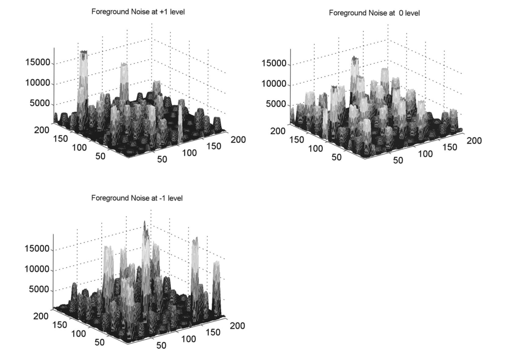
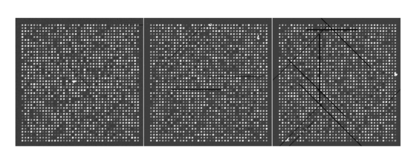
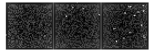
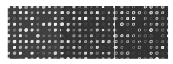
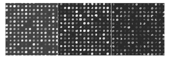
The analysis of a detection algorithm begins with a ground truth. Here that ground truth refers to a “true” expression intensity that must be estimated by the detection algorithm. A microarray containing N gene expression spots with intensity levels I_k, for k=1,…,N, is simulated by an exponential distribution. Base intensities for the red and green channels, R_k and G_k, respectively, are generated from two independent normal distributions having a mean I_k and standard deviation αI_k, where α is a common coefficient of variation.

A particular gene (RNA) may be over/or underexpressed, and this will show up in the red (test) channel. We refer to such a gene as an expresser or outlier. These are found randomly in the model by selecting a gene from the entire microarray with a probability p _outlier to be an outlier. If gene k is selected, then a scaling factor t_k=10^b_k is applied, where b_k satisfies a beta distribution, b_k∼Β(1.7,4.8), and where the ± sign is selected with equal probability. Based on the scaling factor, the individual channel intensities are given by $R_k^{\prime }=R_k\sqrt{t_k}$ and $G_k^{\prime }=G_k/\sqrt{t_k}$

The dyes commonly used for microarray experiments show nonlinear response characteristics, and different dyes give different responses. This effect is modeled by the nonlinear function

Normally distributed foreground noise of intensity I_f is added pixelwise on the spots (simulation 9 in the appendix). This foreground noise typically has zero mean. It results in spot intensities SR=R_k ^″+I_f1 and SG=G_k ^″+I_f2. Figure 2 shows noise addition at various levels. In this figure, and in all subsequent figures illustrating noise, all other noise factors are set at the best level (less variant than +1 level).

Figure 2

Foreground noise variation illustrated at three levels: +1, 0, −1.  

Owing to laboratory dust that may stick on the arrays and fluoresce on laser excitation to give high-intensity spikes, or high-intensity points caused by cDNA precipitation, spike noise, at a preset rate, L_spi, is added randomly across the entire slide area. Once a pixel is selected for spike noise, the adjacent pixels have a higher probability of being affected. This is fixed by a random number chosen from a uniform rate, W_spi, which gives a count of pixels randomly chosen to be influenced by this noise. The intensity, N_S, of the spike noise is governed by an exponential distribution with mean μ_spi. Figure 3 shows spike noise added at different levels.

Figure 3

Spike noise variation illustrated at three levels +1, 0, −1 (left to right).

Physical handling of the array slides can result in scratch noise (surface scratches), which typically results in low intensity levels. Scratch-noise intensity is parameterized as a ratio, κ_sc, giving the background-to-scratch noise intensity level. Other parameters are the number of strips, strip thickness W_sc, and a random strip length, L_sc (simulation 24 in the appendix). These scratches are placed at random positions on the array and are inclined according to a (discrete) uniformly random angle, θ_sc∈{0,45,90,135,180}. Figure 4 shows scratch noise at different levels.

Figure 4

Scratch noise variation illustrated at three levels: +1, 0, −1 (left to right).

Fine dust particles on the slides can create snake noise upon laser excitation. These snake-noise strips are typically of higher intensity than the signal level. To simulate this noise, multidirectional snake noise has been generated consisting of some number, N _seg , of segments. Analogously to scratch noise, the intensity is parameterized as a ratio, κ_sn, giving the average signal-to-snake noise intensity level, the number of snakes, snake thickness W_sn, and a random length, L_sn, given as a multiple of the spot size. Figure 5 shows snake noise at different levels.

Figure 5

Snake noise variation illustrated at three levels +1, 0, −1 (left to right).  

The cDNA deposition spot is considered to be circular, with a random radius S (simulation 1 in the appendix). The mean of the radius is set according to the array density, and its variance relates to the consistency of spot size. The standard deviation is a predetermined proportion, k_s, of the mean. The radius mean is set for every block, and randomized over a small range within the array (simulation 12). Depending on the robot arm and printing ability of the pins, the interspot distance, G_sp, may vary. Owing to the physical mechanics of the robot arm, the block size (pixel units) is fixed in most cases. The interspot distance can be set to accommodate spot size and random variations in spot radii. The spot variability at three levels is shown in Fig. 6.

Figure 6

Spot radius deviation illustrated at three levels: +1, 0, −1 (left to right).

Owing to the impact of the print tip on the glass surface, or possibly to the effect of surface tension during the drying process, a significantly lesser amount of cDNA can be deposited near the spot center. An elliptical shape models this inner hole with random horizontal and vertical axes, H and V (simulation 3). Interarray variability in the distributions of H and V is modeled by uniformly distributed means μ_H and μ_V (simulation 14). The choice of the parameters governs the hole shapes. The center position of a hole is allowed to drift over a range (simulation 4). The shape is unaffected by the drift because the contact of the mechanical print tip to the surface is unaffected. Figure 7 shows the noise at different levels.

Figure 7

Inner hole noise variation illustrated at three levels: +1, 0, −1 (left to right).  

The irregularity of RNA washout during slide preparation is modeled by chord noise (chord removal). The number, N_c, of chords to be removed for a spot is selected from a discrete distribution, {0,1,2,3,4}, where the elements of the distribution occur with probabilities p₀, p₁, p₂, p₃, and p₄, respectively. For images with very few pieces cut off, the zero-chord probability p₀ is very high, and the three- and four-chord probabilities are close to 0 (possibly equal to 0). To model interarray variability, the probabilities can be treated randomly. This noise parameter is set once for every block that is not a spot level noise. Once the number of chords for a spot is determined, the distance, L, of each chord center to the edge is selected from a beta distribution, with interblock variability for the beta distribution being uniformly modeled (simulation 5). Finally, the chord locations are chosen uniformly randomly according to an angle θ between 0 and 2π. Figure 8 shows chord noise at different levels.

Figure 8

Chord noise variation illustrated at three levels: +1, 0, −1 (left to right).

Owing to the manner in which liquid dries, the spots usually do not have smooth edges. Edge noise is simulated via a parameterized edge-noise algorithm adopted from digital document processing. Edge noise is applied to the outer perimeter of the spot (after chord removal). Figure 9 shows the noise at different levels.

Figure 9

Spot edge variation illustrated at three levels: +1, 0, −1 (left to right).

Many factors contribute to the fluorescent background observed: autofluorescence from the glass surface or the surface of the detection instrument, nonspecific binding of fluorescent residues after hybridization, local contamination from posthybridization slide handling, etc. Background noise is simulated by a normal distribution whose parameters are randomly chosen to describe the process, and for multiple arrays, the interarray difference is modeled by a uniform distribution (simulation 20).

Rather than be constant across the entire microarray, the mean of the background noise may vary, owing to various scanning effects. It can take different shapes: parabolic, positive slope, or negative slope. In this case a function g(x,y) is first generated (parabolic, positive slope, or negative slope) to form a background surface and normal noise is added to it pixelwise. Figure 10 shows parabolic background noise at different levels.

Figure 10

Variation in signal-to-background noise ratio (SigBack) and parabolic background. SigBack is set at −1, while parabolic background is varied from +1, 0, −1, left to right.

The addition of various noise types makes the microarray highly peaked, with high pixel differences. This stark irregularity can be mitigated by smoothing the image with either a flat or pyramidal convolution kernel. Our simulation study uses a flat smoothing function.

Once a microarray image has been simulated, the signal extraction toolbox Dearray uses statistical methods to segment the signal and the background pixels.^{6 7} Different levels of significance can be set for this procedure. Once the signal pixels are identified, a trimmed mean of their values gives an estimate of the signal mean. Background information is extracted by taking pixel information from four corners of a given spot to estimate its mean. Actual signal expression is estimated by the difference between the two. If a spot’s irregularity in shape and signal (area of the spot, signal variation, etc.) is reflected by a low-quality metric, then the spot can be flagged. At the final step, a linear corrective normalization procedure is carried out to compensate for variation in the dye response. Ratio intensities are then computed. A logarithmic scale applied to the ratios can be used to map the data to a desirable range.

3.

Experimental Design and Statistical Data Analysis

The array model has more than twenty parameterized noise conditions. We consider thirteen commonly occurring noise conditions for this study. These are grouped into four categories, which then correspond to four experiments: (1) background noise, (2) shape noise, (3) surface noise, and (4) weak signal. Each category has five conditions, with some of the thirteen conditions occurring in more than one category. The experiments are described in Table 2. In experiments 1A through 4A, each factor can take on two levels, 0 or 1. In experiments 1B through 4B, the factors take on the levels −1 or 1. Assuming two levels for each noise factor, there are thirty-two conditions for each category. For each condition, 8 replicate arrays are generated so there are 256 arrays per experiment. Each array has 1600 spots in a 40×40 matrix format. These numbers have been chosen to provide sufficient replicates while not resulting in inordinate image-processing time.

Table 2

4.

Experimental Results

As noted in the introduction, signal-detection algorithms can recover the true signal more easily for images with less severe levels of noise. Thus, when comparing experiments 1A to 4A with experiments 1B to 4B, with the noise level 0 (less severe) and noise level −1 (more severe), respectively, we expect that the true gene expression can be more accurately estimated in experiments 1A to 4A. This means that for data with more noise (−1; experiments 1B to 4B) the difference between the estimated and true expression ratio is greater. This is shown in Fig. 11, where, for all experiments, the distributions of these absolute differences at their most extreme noise level (all 0, or all −1) in log-log scale are presented by box plots. The top and bottom edges of each box correspond to the upper and lower quartiles of the measurements, respectively. The solid dots in the middle give the locations of the medians. Figure 11 clearly shows that the medians and upper quartiles of 1B to 4B are larger than the corresponding medians and upper quartiles of 1A to 4A.

Figure 11

Box plots for absolute differences between the true and estimated expression ratios in a log-log scale. For each experiment, only the responses in the most extreme level (all −1 for Bs and all 0 for As) are plotted. Each box contains the central 50 of the data. The solid dot in the middle gives the location of the median. The top and bottom whiskers reach the largest and smallest nonoutlying observations, respectively, while the circles indicate the locations of outlying observations.

In this paper our interest goes beyond this general statement; it is to determine the kinds of noise reduction that significantly affect signal estimates. For instance, in experiment 1, concerning background noise, if there is a significant difference between levels −1 and 1 for the parabolic background factor (p<0.0033), then lessening the curvature of the parabolic background significantly improves estimation at level α=0.05. We reach this conclusion because the response for the factorial experiment is the absolute difference between the estimated and actual signal values.

Let us consider experiment 1 in detail, the results being given in Table 4. The four columns of the table correspond to experiment 1B for all signal levels, 1B for low signal levels, 1A for all signal levels, and 1A for low signal levels. For each experiment, data in the low signal level comprise the one-third of the original data points whose true signal values are in their lower tertile. We have considered low signal levels as a case in their own right (besides being included among all signal levels) because signal detection is made more difficult when a signal is low. The table is broken into main effects and interactions. For experiment 1B (level −1 versus level 1) using all signals, all five effects are significant. This means that reducing any of these effects can be helpful. They are also all significant for low signals. Note that all five factors in the experiment directly affect pixel values, either raising or lowering them for the affected pixels, and the difference in degrees between levels −1 and 1 significantly affects signal estimation. The magnitude of the t-test statistics suggests that the high outlier and spike noise levels are more damaging to the image than the others.

Table 4

If we now consider experiment 1A (level 0 versus level 1) for all signals, both spike and snake effects become insignificant. This means that, relative to snake or spike noise, signal estimation is not significantly different at these two levels. Looking at the fourth column, we see that spike noise is still significant for level 0 versus level 1 for low signals. For these, there is a significant difference in performance of the algorithm relative to spike noise.

Interpretation of interactions can often be difficult, but in some cases it can be revealing. For instance, confining ourselves to the case of all signal levels, in experiment 1B we see that there is interaction between the signal-to-background noise and the parabolic effect. This is not surprising because the ratio is affected by the background. The interaction of the outlier effect and spike noise is also reasonable since both produce extreme values on the microarray. The large positive t-test statistic suggests a strong “synergistic” interaction effect throughout all four scenarios. A similar type of interaction is observed when both signal-to-background noise and parabolic-background noise levels are high. Figures 12 and 13 illustrate the mixed visual effects between signal-to-background noise and parabolic-background noise and spike noise, respectively, with the underlying true spot-intensity distributions being the same in each part and with only the noise factors contributing to the differences.

Figure 12

Signal-to-background and parabolic noise at (+1,+1), (0,0), (−1,−1) level, from left to right.  

Figure 13

Signal-to-background and spike noises at different levels.

For experiment 2 (shape noise), in Table 5 we see that four of the factors are significant for experiment 2B, for all signals or just low signals. Among them, the strongest factors are the inner hole size and the foreground noise. The effect of foreground noise is similar to background noise in that it directly affects pixel values. The effect of low spot radius, large inner hole size, and excessive chord removal is to lessen the signal area, thereby reducing the pixel area over which the signal is to be estimated. Chord removal is not significant in experiment 2A for low signals, which means that at level 0 there is insufficient chord removal to significantly affect signal estimation relative to level 1. The fact that edge noise is not significant in experiment 2B indicates that the imaging algorithm can deal equally well with spot detection at both levels relative to handling edge noise.

Table 5

There is an apparent anomaly with regard to edge noise in experiment 2A: edge noise is significant relative to levels 0 and 1, but not with respect to levels −1 and 1. This phenomenon is an “apparent” anomaly because one cannot compare p values across different experiments with full confidence—although we often do make such comparisons in a heuristic mode. Recall that the denominator of the F-statistic contains a variance estimator, and therefore a low variance will tend to make the F-statistic significant. Because the variance is very low in experiment 2A in contrast to experiment 2B, significance in the former and lack of significance in the latter is a reasonable consequence and does not imply that the difference in damage between two levels in experiment 2B is less than that in 2A. The damage effect of edge noise starts to show in 2A when the effects of inner hole size and foreground noise are not as dominating as they are in 2B. In experiment 2B, the effect of edge noise is still present in its significant interaction with both spot radius and chord noise. Figure 14 shows the mixed visual effect between the spot radius and chord noise.

Figure 14

Spot radius deviation and chord noise at (+1,+1), (0,0), (−1,−1) levels, from left to right.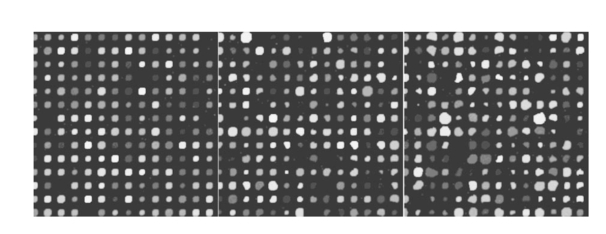

Regarding interaction in experiment 2B, the three distinctly geometric factors (spot radius, inner hole, and chord noise) interact significantly for both the overall signal and low-signal cases. This is reasonable because each affects the area over which signal estimation takes place. Interaction is greatly reduced in experiment 2A, particularly for low signals, where only interaction between the inner hole and chord removal is strongly significant. Figures 15 and 16 show the mixed visual effects of the inner hole with spot radius and chord noise, respectively.

Figure 15

Spot radius deviation and inner hole at (+1,+1), (0,0), (−1,−1) levels, left to right.

Figure 16

Inner hole and chord noises at (+1,+1), (0,0), (−1,−1) levels, left to right.  

Whereas experiment 2 mixes shape effects with foreground noise and edge noise, experiment 3 mixes them with scratch and snake noise. Table 6 shows a fair amount of consistency between the two experiments with regard to the three geometric factors relative to both main effects and interaction. One notable change is that the interaction between spot radius and chord removal changes from being “antagonistic” in experiment 2 to being “synergistic” in experiment 3. Even though the order of estimated cell means in the four noise level combinations remains the same in both experiments, in experiment 3 the estimated cell mean when both noise factors are present is much higher than in the other three; consequently, a significant “synergistic” interaction is observed. For the most part, snake and scratch noise show no significant main effects. The exception is scratch noise for low signals in experiment 3B. This is quite plausible because scratch noise causes a strip of low values, thereby reducing an already low signal. Note also the interaction of snake and scratch noise in three of the four experiments.

Table 6

Experiment 4 concerns signal conditions, in particular, signal deviation, signal-to-background ratio, and foreground noise. These conditions are bound to affect signal estimation, and the main-effects part of Table 7 demonstrates this. The only exception is for low-signal values when comparing levels 0 and 1 in experiment 4A. Since signal deviation is tied to the signal mean, a low signal diminishes this deviation and signal deviation is not significant for low signal values. Figure 17 shows the mixed visual effects between signal-to-background and spike noise. As has been common throughout, overall interaction between the factors is much less relative to levels 0 and 1 than with respect to levels −1 and 1.

Figure 17

Signal-to-background and spike noise variation at (+1,+1), (0,0), (−1,−1) levels, left to right.

Table 7

5.

Conclusion

Factorial analysis has been applied to simulated microarray images to study the effects and interaction of noise types at different noise levels. This type of analysis provides a general paradigm for investigating the effects of noise within a comprehensive simulation environment, thereby providing a tool by which one can quantitatively determine which kinds of noise should be mitigated in microarray technology. For instance, from the analysis described in this paper, it can be concluded that elimination of the inner hole and the stabilizing of spot radius will have a strongly beneficial effect on signal estimation. Additional information can be found online.¹⁴

Appendix

Parameter settings for the microarray simulation. The notation N(a,b) denotes the normal distribution with mean a and variance b; U[a,b] is the uniform distribution on the interval [a,b]; U{a,b,c,…} is the uniform distribution on the indicated set of values; Β(a,b) is the beta distribution with parameters a and b; and exp(a) is the exponential distribution with mean a.