Wavelet analysis of two-dimensional birefringence images of architectonics in biotissues for diagnosing pathological changes

Oleg V. Angelsky; Gennadiy V. Demyanovsky; Alexander G. Ushenko; Dimitry N. Burcovets; Yuriy A. Ushenko

doi:10.1117/1.1755720

1 July 2004 Wavelet analysis of two-dimensional birefringence images of architectonics in biotissues for diagnosing pathological changes

Oleg V. Angelsky, Gennadiy V. Demyanovsky, Alexander G. Ushenko, Dimitry N. Burcovets, Yuriy A. Ushenko

Author Affiliations +

Journal of Biomedical Optics, Vol. 9, Issue 4, (July 2004). https://doi.org/10.1117/1.1755720

Abstract

A method for polarization filtering, correlation processing, and wavelet analysis of coherent images of physiologically normal and necrotically changed (myocardium infarct) muscle tissue is presented. A technique for early optical diagnosis of the appearance of these biological tissues and the course of their degenerative-dystrophic changes is proposed.

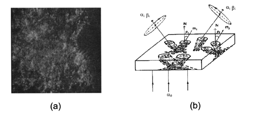
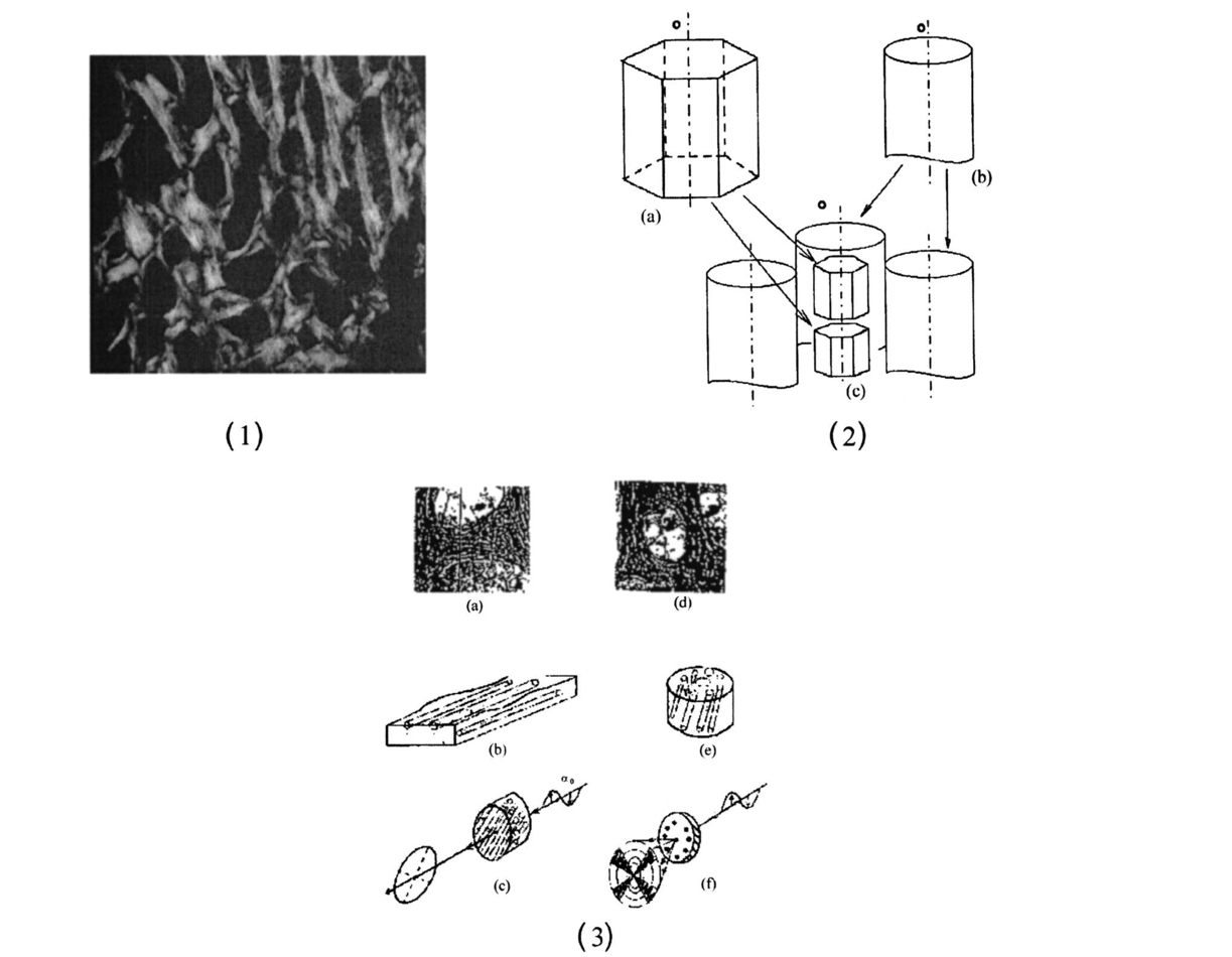
1. Introduction

This paper discusses the vector structure of the laser fields of objects formed by biological tissues, and the development of optical diagnostics for their physiological state through correlation processing and wavelet analysis of corresponding polarization images. Histological sections of physiologically normal muscle tissue (group a) and necrotically changed (myocardium infarct) tissue (group b) of a rat’s heart were studied.

2. Theoretical Modeling

2.1.

General Remarks

On the basis of information on the morphological structure of biotissue,¹ the following model scheme is suggested. Biotissue generally consists of two phases: amorphous and optically anisotropic phases. The optically anisotropic component has two levels of organization: crystalline and architectonic.² Optically coaxial organic fibrils that form collagen, elastin, myosin fibers, mineralized (hydroxyapatite crystals) and organic fibers, etc. can be included in the crystalline level. Spatially determined (muscle tissue, vessel walls, tunics of organs, bone plates, etc.) and statistically disordered bundles (spongy bone tissue, soft tissues, miometry, skin derma etc.) form architectonics of the biotissue. The architectonic nets of such biotissues as skin derma (SD), muscle (MT), and bone tissues (BT) are morphologically the most typical ones.

The architectonics of skin derma is formed by statistically oriented bundles of collagen fibrils (Fig. 1). The diameter of the fibrils ranges from 0.5 to 2 mcm. Parallel bundles of fibrils form a fiber, the diameter of which is 5 to 7 mcm (papillary layer),³ and in the net layer it reaches 30 mcm.³ A collagen bundle, the average diameter of which changes from 100 to 200 mcm, is considered to be the highest structural unit of optically active collagen (birefringence value Δn≈10⁻³) .⁴

Figure 1

Model representation of skin derma architectonics.

Bone tissue represents a system consisting of the trabeculae and osteons [Fig. 2(1)]. The optically active matrix consists of hydroxyapatite crystals (Δn≈10⁻¹), ² the long (optical) axes of which are directed along the longitudinal axis of collagen fibers [Fig. 2(2)]. They are located between microfibrils, fibrils, and collagen fibers forming a separate continuous mineral phase. Collagen fibers are spatially armoring elements in mineral matrix. The orientation of bone trabeculae fibers is ordered and parallel to their plane [Fig. 2(3)]. Bone tissue osteons have a spatially spiral orientation of the armoring collagen fibers.

Figure 2

Model representation of bone tissue structure.

Muscle tissue is a structured, spatially ordered system of protein bundles consisting of optically isotropic actin and anisotropic myosin⁴ (Fig. 3).

Figure 3

Model representation of muscle tissue structure.

2.2.

Optical Characteristics

The optical properties of the primary (crystalline) level of BT organization are characterized by a Mueller operator of the following kind.⁵

Eq. (1)

{Q} = ‖ \begin{matrix} 1; & 0; & 0; & 0; \\ 0; & ({sin}^{2} \frac{δ}{2} \times cos 2 ρ + {cos}^{2} \frac{δ}{2}); & (0.5 sin 4 ρ {sin}^{2} \frac{δ}{2}); & (- sin 2 ρ sin δ); \\ 0; & (0.5 sin 4 ρ {sin}^{2} \frac{δ}{2}); & (- {sin}^{2} \frac{δ}{2} \times cos 2 ρ + {cos}^{2} \frac{δ}{2}); & (cos 2 ρ sin δ); \\ 0; & (sin 2 ρ sin δ); & (- cos 2 ρ sin δ); & (2 {cos}^{2} \frac{δ}{2} - 1) . \end{matrix} ‖ .

Here the ρ orientation of the optical axis created by the packing direction of anisotropic fibrils (collagen, myosin, elastin, hydroxyapatite, etc.), δ-value of phase shift, performed by their substance between ordinary and nonordinary waves, x, y coordinates in the BT sample plane.

Within the crystalline domain, the orientational ρ and δ phase parameters are either typologically stationary [ρ(x,y),δ(x,y)≈const] or determinedly distributed. In the first case, the polarization state of the laser field (azimuth α and ellipticity β) of the crystallite domain is determined by solving the following matrix equation⁴:

Eq. (2)

\begin{matrix} M & = & ‖ \begin{matrix} 1 & 0 & 0 & 0 \\ 0 & {cos}^{2} 2 ρ + {sin}^{2} 2 ρ cos δ; & sin 2 ρ cos 2 ρ (1 - cos δ); & - sin 2 ρ sin δ; \\ 0 & {sin}^{2} ρ {cos}^{2} ρ (1 - cos δ); & {sin}^{2} 2 ρ + {cos}^{2} 2 ρ cos δ; & cos 2 δ sin δ; \\ 0 & sin 2 ρ sin δ; & - cos 2 ρ sin δ; & sin δ . \end{matrix} ‖ \cdot (\begin{matrix} 1 \\ cos 2 α_{0} \\ sin 2 α_{0} \\ 0 \end{matrix}) \\ = & (\begin{matrix} 1 \\ ({cos}^{2} 2 ρ + {sin}^{2} 2 ρ cos δ) cos 2 α_{0} + sin 2 ρ cos 2 ρ (1 - cos δ) sin 2 α_{0} \\ sin 2 ρ cos 2 ρ (1 - cos δ) cos 2 α_{0} + ({sin}^{2} 2 ρ + {cos}^{2} 2 ρ cos δ) sin 2 α_{0} \\ sin 2 ρ sin δ cos 2 α_{0} - cos 2 ρ sin δ sin 2 α_{0}, \end{matrix}), \end{matrix}

where α₀ is the polarization azimuth of the laser beam that illuminates the biotissue. It follows from Eq. (2):

Eq. (3)

α = \frac{1}{2} arctan \frac{sin 2 ρ cos 2 ρ (1 - cos δ) cos 2 α_{0} + ({sin}^{2} 2 ρ + {cos}^{2} 2 ρ cos δ) sin 2 α_{0}}{({cos}^{2} 2 ρ + {sin}^{2} 2 ρ cos δ) cos 2 α_{0} + sin 2 ρ cos 2 ρ (1 - cos δ) sin 2 α_{0}};

Eq. (4)

β = \frac{1}{2} arcsin [sin δ \times sin 2 (ρ - α_{0})] .

For a flat-polarized wave with azimuth α₀=0 deg, expressions (3) and (4) are transformed:

Eq. (5)

α = \frac{1}{2} arctan [\frac{sin 2 ρ cos 2 ρ (1 - cos δ)}{{cos}^{2} 2 ρ + {sin}^{2} 2 ρ cos δ}];

Eq. (6)

β = \frac{1}{2} arcsin (sin δ \times sin 2 ρ) .

In the second case (curvilinear packing of fibrils described by a curve of the second order (A₁x²+C₁y²+2D₁x+2E₁y+F₁=0), the polarization characteristics of the object field continuously change at every point (x_i,y_i) and are determined by relations that are analogous to Eqs. (3) to (6). The difference is that the angle ρ gives the sense of angle ω=g(x,y) between the tangent to the curve at point (x_i,y_i) and the polarization azimuth of the laser beam α₀.

Thus, for some types (circle, ellipse, parabola, hyperbola) of fibril packing, it can be shown that in the x direction the functions g(x,y) give the following form:

Eq. (7)

ω = arctan \frac{\sqrt{r^{2} - x^{2}}}{x},

Eq. (8)

ϖ = a r c t a n \frac{(a^{2} - b^{2}) \times \sqrt{a^{2} - x^{2}}}{a^{3} b \times x},

Eq. (9)

ϖ = arctan \frac{\sqrt{c^{2} - x^{2}} (c^{2} - 2 d^{2} x)}{c d^{2} (c^{2} + d^{2} x^{2})},

Eq. (10)

ϖ = \frac{x^{2}}{k},

where r is the radius of the circle; a and b are the large and small half-axes of the ellipse; and c, d, and k are the coefficients of the hyperbola and parabola, respectively.

For an architectonic net of BT, the vector structure of the object field can be defined as the superposition of polarization states of the crystalline domains:

Eq. (11)

α^{*} = arctan (\frac{Σ_{m = 1}^{N} Σ_{n = 1}^{N} A_{m} cos α_{n}}{Σ_{m = 1}^{N} Σ_{n = 1}^{N} A_{m} sin α_{n}}),

Eq. (12)

β^{*} = arctan [\frac{Σ_{m = 1}^{N} Σ_{n = 1}^{N} Σ_{r = 1}^{N} A_{m} (cos α_{n} + tan β_{r} sin α_{n})}{Σ_{m = 1}^{N} Σ_{n = 1}^{N} Σ_{r = 1}^{N} A_{m} (s i n α_{n} + t a n β_{r} c o s α_{n})}],

where N is the number of anisotropic structures and A_m is the amplitude of light oscillations of partial object fields.

2.3.

Structural Architectonic Nets of BT

For most biotissues, the substance of optically anisotropic architectonics is of the same type. That is why it can be considered that Δn=const. On the other hand, such an approximation is not always adequate. Thus, for an anisotropic component of bone tissue, nonorganic crystals of hydroxyapatite and collagen fibrils are the main optically active structures. The spatial symmetry of the crytalline structure of the nonorganic and organic microcomponents of bone tissue is identical these are optically coaxial crystals.⁵ Consequently, their joint effect on the photometric and polarization characteristics of optical radiation can be expressed by the superposition of matrix operators of {Q} type [relation (1)].

Eq. (13)

{Q} = {Q}_{1} + {Q}_{2} .

Let us consider the mechanisms of forming the polarization structure of an object field using the example of muscle tissue’s architectonics. Muscle tissue is known to be a structured system of protein fascicles consisting of optically isotropic actin and anisotropic myosin.⁶ The optical properties of this system can be described best by the superposition of a matrix operation of amorphous and crystalline components:

Eq. (14)

\begin{matrix} {M} & = & {A} + {K} \\ = & ‖ \begin{matrix} a_{11} + k_{11} & a_{12} & 0 & 0 \\ a_{21} & a_{22} + k_{22} & k_{23} & k_{24} \\ 0 & k_{32} & a_{33} + k_{33} & k_{34} \\ 0 & k_{42} & k_{43} & a_{44} + k_{44} \end{matrix} ‖ \end{matrix},

where a_ik and κ_mn are elements of partial Mueller matrices of the actin and myosin components of biological tissue.⁵

As a laser beam polarized with an azimuth α₀ passes through this structure, an object field with the polarization state is formed.

Eq. (15)

α = 0.5 arctan [\frac{cos 2 α_{0} k_{32} + sin 2 α_{0} (a_{33} + k_{33})}{a_{21} + cos 2 α_{0} (a_{22} + k_{22}) + sin 2 α_{0} k_{23}}],

Eq. (16)

β = 0.5 arcsin (cos 2 α_{0} + sin 2 α_{0} k_{43}) .

The spatial intensity distribution of this field, which is observed through an analyzer oriented at an angle Ω relative to the plane of incidence, can be written as follows:

Eq. (17)

I (X, Y) = I_{0} {{cos}^{2} (α - Ω) + {sin}^{2} (α - Ω) {tan}^{2} β} .

On the other hand, this field is formed by the superposition of two components:

Eq. (18)

I (x, y) = Ψ (x, y) + T (x, y),

where Ψ(x,y) and T(x,y) are the field components formed by the myosin and actin components of muscle tissue, respectively.

It follows from the analysis of relations (14) to (17) that the vector structures of images of these components are fundamentally different. The object field of the actin component is linearly polarized. Therefore the intensity of the T(x,y) component can be practically reduced to zero by using an analyzer oriented at the angle

Eq. (19)

Ω^{*} = \frac{π}{2} + 0.5 arctan (\frac{sin 2 α_{0} a_{33}}{a_{21} + cos 2 α_{0} a_{22}}) .

In this case, a system of polarizophots (zero-intensity lines) is formed. The corresponding intensity distribution in a coherent image of the actin component of muscle tissue varies to the level determined by the relation

Eq. (20)

Ψ^{*} (X, Y) = 0.25 Ψ (X, Y) \times {{cos}^{2} [\frac{sin 2 α_{0} k_{33} + cos 2 α_{0} k_{32}}{sin 2 α_{0} k_{33} + cos 2 α_{0} k_{22}}] + {sin}^{2} [\frac{sin 2 α_{0} k_{33} + cos 2 α_{0} k_{32}}{sin 2 α_{0} k_{32} + cos 2 α_{0} k_{22}}]} .

The relation between the concentrations of myosin and actin protein components and their biochemical exchange plays a major role in the mobility and contraction of muscle tissue, which is one of the decisive factors in its vital activity. Pathological changes in this biological tissue are accompanied by the reduction or disappearance of actin proteins, leading to the dystrophy or necrosis (myocardium infarct) of muscles.⁷

The early optical diagnostics of these processes can be represented by the following stages: formation of a noncoherent image of muscle tissue, polarization selection of this image with the subsequent visualization of the myosin and actin components, correlation processing of the corresponding polarization images, and wavelet analysis of their structures.

3. Correlation Processing of Polarization Components of Coherent Images of Muscle Tissue

Laser radiation propagating through a biotissue produces a coordinate-distributed optical signal S(X,Y):

Eq. (21)

S (X, Y) = I (X, Y) + U (X, Y),

where U(X,Y) and I(X,Y) are the random and anisotropic (informative) parts of the object field. These quantities can be generally represented as a superposition of random I^*(X,Y) and stochastic I^*(X,Y) (quasi-regular) components:

Eq. (22)

I (X, Y) = I^{*} (X, Y) + I^{\otimes} (X, Y) .

Let us use an autocorrelation to consider the possibility of detecting and analyzing the multifractal component in a coherent image of a biotissue against a background related to the amorphous component. For the simplicity of our analysis, we restrict our consideration at the initial stage to the one-dimensional case. The autocorrelation function in this case is defined by the following expression:⁸

Eq. (23)

G_{x x} (Δ x) = lim_{x \to \infty} \frac{1}{X_{0}} \int_{0}^{x} [I (X) + U (X)] [I (X - Δ X) + U (X - Δ X)] d x .

Since the correlation operator is distributive, we find that

Eq. (24)

G_{x x} (Δ x) = G_{i i} (Δ x) + G_{u u} (Δ x) + G_{i u} (Δ x) + G_{u i} (Δ x) .

Let us assume that the noise U(X) and the signal I(X) are independent. Then the correlation functions G_iu(ΔX) and G_ui(ΔX) are identically equal to zero (with an accuracy up to the errors arising from the finiteness of the integration interval). Therefore Eq. (24) can be rewritten as

Eq. (25)

G_{x x} (Δ x) = G_{i i}^{*} (Δ x) + G_{u u}^{*} (Δ x) + G_{i i}^{\otimes} (Δ x) + G_{u u}^{\otimes} (Δ x) .

The autocorrelation noise functions G_ii ^⊗(Δx); G_uu ^⊗(Δx) tend to zero as the interval X₀ increases.⁸ Thus two terms survive in the expression for the autocorrelation function of the multifractal component in the coherent image of a biotissue:

Eq. (26)

G_{x x} (Δ x) = G_{i i}^{*} (Δ x) + G_{u u}^{*} (Δ x) .

The term G_uu ^*(ΔX) plays the role of an error in the definition of G_xx(ΔX). Generally, we have G_ii ^*(ΔX)≈G_uu ^*(ΔX). Therefore the selection of the autocorrelation function G_ii ^*(ΔX), which is important for diagnostic purposes, is not sufficiently efficient.

3.1.

Computer Modeling

The solution of this problem can be optimized through the polarization selection of the coherent image of the biotissue under study. In such a situation, the analytical expression for the object signal in Eq. (22) takes the following form:

Eq. (27)

S^{*} (x) = I^{*} (x) + I^{\otimes} (x),

and the autocorrelation function:

Eq. (28)

G^{*} (Δ x) = lim_{x \to \infty} \frac{1}{X_{0}} \int_{0}^{x} W (α) V (β) {[{sin}^{2} α (x) + t g^{2} β (x) {cos}^{2} α (x)] \times [{sin}^{2} α (x - Δ x) + t g^{2} β (x - Δ x) {cos}^{2} α (x - Δ x)]} d x .

It can be seen that Eq. (27) illustrates the possibilities of autocorrelation in determining the architectonic component of a coherent image of a biotissue.

According to the Wiener-Khinchin⁸ theorem, in estimating such a component it is convenient to use the algorithm for determining its spectral density:

Eq. (29)

S_{x x} (v) = \int_{- \infty}^{\infty} G_{x x}^{*} (Δ x) c o s (2 π v x) d x,

where v is the spatial frequency.

It follows from the analysis in Eqs. (28) and (29) that the appearance of pathological changes leading to changes in the direction of growth in the architectonic structure of biotissues (tumorlike processes) is connected with the appearance of a quasi-linear spectrum S_xx(v). In contrast, the destruction of the architectonic net (osteoporosis, rachitis, etc.) is accompanied by the formation of a continuous spectrum S_xx(v).

Figure 4 illustrates the tendencies of changes in the autocorrelation functions G_xx(Δx) and the corresponding densities S_xx(v), which are obtained from the algorithms in Eqs. (28) and (29), for the corresponding values of the orientation parameters of an architectonic net that contains the harmonic component v:

Figs . 4 (a) and 4 (b) ρ_{0} = 45 deg; σ_{ρ} = 5 deg

Figs . 4 (c) and 4 (d) ρ_{0} = 45 deg; σ_{ρ} = 45 deg

Figs . 4 (e) and 4 (f) ρ_{0} = 45 deg; σ_{ρ} = 90 deg

It can be seen that the effectiveness of differentiating the harmonious component in the intensity distribution of a coherent image is the greatest for σ_ρ=5 deg and, vice versa, the least for σ_ρ=90 deg.

Figure 4

Autocorrelation functions and spectral densities of computer-simulated signals. See text for explanation.

3.2.

The Technique of Calculating Autocorrelation Functions of Biotissue Architectonic Images

This method is based on the determination of the autocorrelation coefficient of spatial intensity distributions of the partial image components Ψ(X,Y) and T(X,Y) obtained experimentally in various polarizations⁹:

Eq. (30)

r = \frac{σ_{Ψ, \tilde{ψ}}}{σ_{ψ} σ_{\tilde{ψ}}},

where σ_Ψ,ψ˜ is the covariance of two intensity arrays in the coherent image of biological tissue, the autocorrelation of which is studied, and σ_Ψ and σ_Ψ˜ are the intensity dispersions:

Eq. (31)

σ_{ψ, \tilde{ψ}} = \frac{1}{m n} \sum_{i = 0}^{m - 1} \sum_{j = 0}^{n - 1} (ψ_{i, j} - \bar{ψ}) ({\tilde{ψ}}_{i, j} - \bar{\tilde{ψ}}),

Eq. (32)

σ_{ψ}^{2} = \frac{1}{m n} \sum_{i = 0}^{m - 1} \sum_{j = 0}^{n - 1} {(Ψ_{i, j} - \bar{Ψ})}^{2},

Eq. (33)

σ_{\tilde{Ψ}}^{2} = \frac{1}{m n} \sum_{i = 0}^{m - 1} \sum_{j = 0}^{n - 1} {({\tilde{Ψ}}_{i, j} - \bar{\tilde{Ψ}})}^{2},

Eq. (34)

\bar{Ψ} = \frac{1}{m n} \sum_{i = 0}^{m - 1} \sum_{j = 0}^{n - 1} Ψ_{i, j}, a n d

Eq. (35)

\bar{\tilde{Ψ}} = \frac{1}{m n} \sum_{i = 0}^{m - 1} \sum_{j = 0}^{n - 1} {\tilde{Ψ}}_{i, j} .

The calculated collection of correlation coefficients for each sampling of the intensity array in the horizontal and vertical directions of the analysis form the autocorrelation function G(ψψ) of the polarization pattern of the laser image of biological tissue.

4. Wavelet Analysis of Polarization Images of Biological Tissue

A wavelet transformation of the object field consists in its expansion by a certain basis, which is constructed of a solitonlike (wavelet) function by way of its scaling and transfer. Each function of this basis characterizes a certain spatial frequency as well as its spatial localization in a coherent image of biological tissue.¹⁰ Thus, the following new possibilities appear in addition to correlation analysis:

• determining the space-distributed properties of the object field of the investigated biotissue
• differentiation of alternation and dissipation areas
• obtaining local high-frequency and global large-scale information on the biotissue’s structure

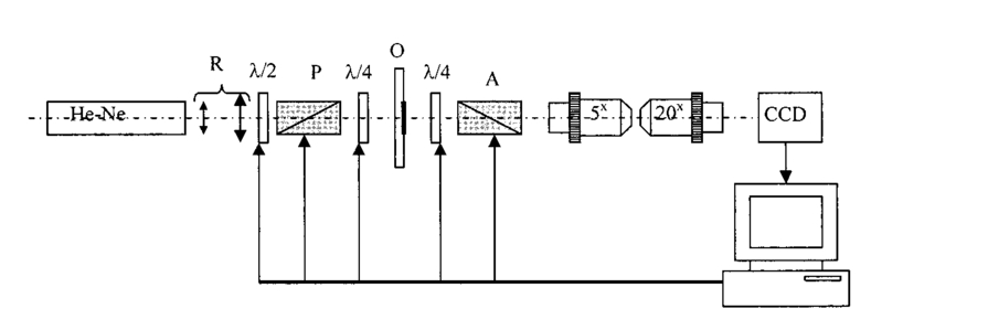
This is why the wavelet analysis can be regarded as a “mathematical microscope.” The ability of such a “microscope” to detect the inner structure of a sufficiently inhomogeneous object and to study the local scaling properties is shown by many examples: the Weierstrasse fractal function, probabilistic measures of Cantor sets, multifractal measures of several well-known dynamic systems, and modeling the situations of change to chaos observed in dissipative systems.¹⁰

Thus the intensity distribution of the object field can be represented as the following series:

Eq. (36)

Ψ (X) = \sum_{j, k = - \infty}^{\infty} c_{j k} ξ_{j k} (X) .

The distribution Ψ(X) belongs to the space L²(R) where it is defined over the entire real axis R(−∞,+∞) and is determined by the finite energy (norm)

Eq. (37)

E_{f} = \int_{- \infty}^{\infty} | Ψ {(X)}^{2} | d x < \infty .

The “waves” forming the space L²(R) are called wavelets ε_ik. They are spatially localized and have a great tendency to decrease to 0. By using discrete scale transformations (1/2^j) and shifts (k/2^j) it is possible to describe all the frequencies and cover the entire axis with the help of one basis wavelet ξ(x).

The basis of the functional space L²(R) can be constructed by using scalings and transfers of the wavelet ξ(X) with arbitrary values of basis parameters, namely, the scaling coefficient a and the transfer parameter b:

Eq. (38)

ξ_{a b} (X) = | a^{- 1 / 2} | ξ (\frac{X - b}{a}); a, b \in R; ξ \in L^{2} (R) .

Based on this, the integral wavelet transformation takes the following form:

Eq. (39)

\begin{matrix} [W_{ξ} W] (a b) & = & {| a |}^{- 1 / 2} \int_{- \infty}^{\infty} Ψ (X) ξ^{*} (\frac{X - b}{a}) d x \\ = & \int_{- \infty}^{\infty} Ψ (X) ξ_{a b}^{*} (X) d x . \end{matrix}

The coefficients c_ik=〈Ψ,ξ_jk〉 of expansion in Eq. (36) of the function Ψ in series in wavelets can be defined through the integral wavelet transformation:

Eq. (40)

c_{j k} = [W_{ξ} Ψ] (\frac{1}{2^{j}}, \frac{k}{2^{j}}) .

If we follow the above-mentioned analogy with the “mathematical microscope,” then the shift parameter b fixes the focusing point of the microscope; the scale coefficient a is the magnification; and finally, by choosing the basic wavelet ψ the optical properties of the microscope are determined.

Basic wavelets are often constructed on the basis of the Gauss function. Among them the complex (Morlett) wavelets and real bases (Mexican hat, MHAT) can be observed. The first ones are well matched to the analysis of the complex signals or fields. As a result of the wavelet transform, the two-dimensional arrays of absolute values and phase are obtained. The application of the MHAT wavelet for analyzing the intensity distribution of coherent images of biotissues is preferable. It has a narrow energy spectrum and two moments (zero and the first ones) that are equal to zero, and it is well matched to an analysis of the scale-coordinate structure of optical fields.¹⁰ That is why in this paper we used the solitonlike function MHAT.¹⁰

It should be pointed out that this choice is not an exclusive one. There exists a wide class of wavelets, the choice of which is determined by the type of information one needs to extract from 1-D or 2-D signals. Optimization of the wavelet-function choice represents a separate problem that is not considered in the paper.

4.1.

Computer Modeling

In order to determine the diagnostic possibilities of wavelet analysis in revealing image anomalies in the first stage, computer modeling of the corresponding situations has been performed. Figure 5 presents a series of images of wavelet coefficients c_ik, given in the axes “coordinate (b)-scale parameter (a).” The following harmonic was used as an analyzed signal I(x):

Eq. (41)

I (X) = {\begin{matrix} I_{0} sin 2 π v x; x_{1} < x < x_{2} \\ I_{0}^{*} sin 2 π v x; x ⩽ x_{1}, x ⩾ x_{2} \end{matrix} .

For pathology in biotissue architectonics, I₀<I₀ ^*; for degenerative-dystrophic changes, I₀>I₀ ^*.

Figure 5

Diagnostic possibilities of wavelet analysis of image anomalies.

From the data obtained it can be seen [Figs. 5(a) and 5(c)] that coefficients c_jk are harmoniously distributed on the interval x₁<x<x₂ and possess a localized extremum corresponding to the coefficient a₀, determined by frequency v, and an extrema in the field of large scales, giving rise to the size b₀, which corresponds to “multifrequent” parts of I(x) distribution (fragments 1 and 2 in Fig. 5). For the “anomalies” there is a change in the value of the wavelet coefficients that is linearly connected with the change in I₀ ^* amplitude. That is why we will use the correlation of the wavelet coefficient levels for the different values of a and b parameters as a criterion to determine the areas of localization of extreme values of the biotissue image intensity.

For a frequency-modulated signal I(x) the transformation of the wavelet coefficients is observed. It consists in redistribution of their amplitudes and an increase in the corresponding interval of scale coefficients a_i [Figs. 5(c) and 5(d)]. However, the parts of the image that show an anomaly of a pathological type are characterized by large amplitudes c_jk and interval a_i. For a model showing a degenerative-dystrophic change in biotissue there is a decrease in c_jk values in the field of small a_i and, vice versa, an increase in the field of large scales. Thus the dispersion of the wavelet coefficients for the corresponding scales has extreme values. It can be regarded as an additional criterion for determining the localization of anomalies in image intensities.

Thus computer modeling data proved the effectiveness of the diagnostic use of wavelet transform in analyzing spatial localization and the anomalous character of the image intensity distribution of harmonious and quasi-harmonious model structures.

5. Automatic Polarimeter Design

The function of the polarimeter is to test the structural elements of the anisotropic tissues acquired by a conventional biopsy method. The overall layout of the instrument is shown in Fig. 6. The main optical elements of the polarimeter are the helium:neon (He:Ne) laser (λ=0.6328 μm, 10 mW), the polaroid (P), two quartz-made quarter-wave (λ/4) plates (4th order) and the polaroid (A) as the analyzer. By setting the polarization plane of P parallel to the optical axis of the first quarter-wave plate, the object under test (O, a tissue sample) is illuminated by a linearly polarized light beam. With the analyzer similarly coupled with the second quarter-wave plate, the isoclines can be analyzed. For that purpose the analyzer has its transmittance plane perpendicular to that of the analyzer (in that case, with no anisotropic object present, the light behind the analyzer is completely extinguished). The isoclines form the set of lines (fringes) over the object area representing the geometric locus of the local optical axis orientations parallel to the plane of polarization of the incident beam.

Figure 6

Scheme of experimental set.

By setting the optical axes of both quarter-wave plates at 45 deg to the linear polarization plane of the light beam, the circular polarization in front of the object under test is obtained. Now the isochromatic lines (the family of lines corresponding to constant phase differences introduced by anisotropic elements found in biotissue) can be studied.

The He:Ne laser beam is expanded by the afocal system R up to a diameter of 3 mm. The pinhole located in the expansion optics removes the scattered light originating from secondary reflections in the resonator and optics contaminations. The role of the half-wave plate λ/2 is to match the laser beam polarization plane to the polarizer transmittance direction and at the same time control the light level at the CCD matrix to avoid its saturation.

The tissue sample is placed on the microscope slide and covered with the microscope cover glass. The slide with tissue is fixed in a mount that provides transverse translations in two mutually perpendicular directions in the range of 5 mm to enable choosing various fragments of the sample.

The sample image is formed on the CCD matrix by an optical system composed of two microscope objectives. The lateral magnification of the imaging system dictated by the matrix and the lateral dimensions of object under test is equal to 4. The overall dimensions of the quarter-wave and analyzer driving systems do not allow placing the imaging optics closer than 200 mm from the sample. Introducing any optical element in front of the analyzer is not recommended since even its residual-level birefringence would cause measurement error. The set of two microscope objectives permits the lateral magnification factor mentioned above to be obtained without the necessity of an excessive axial elongation of the imaging optics. The images registered by the CCD matrix and the frame grabber are transferred in digital form to the computer memory.

The half-wave plate, both quarter-wave plates, the polarizer, and analyzer are rotated by means of step motors. One motor step corresponds to 22.5 min of arc of the rotation of an optical element. The motors are controlled by a D/A card housed in the computer. Two operation modes are possible: automatic mode according to the software developed and manual mode using the keyboard.

Before making measurements, the automatic system is calibrated in the following order:

• The optical axes of quarter-wave plates are set parallel to the transmittance directions of the polarizer and analyzer.
• The transmittance planes of the polarizer and analyzer are set parallel.
• The half-wave plate is rotated to obtain the maximum signal level registered by the CCD matrix (without saturation).
• Both the analyzer and the second quarter-wave plate are rotated into the crossed position with the polarizer.

After a sample is inserted and its image area selected the measurement procedure consists of the following tasks:

• Studies of isoclinic lines: With the polarizer and analyzer crossed (the quarter-wave plates are coupled with the polarizer and analyzer, the tissue sample is illuminated by linearly polarized light), the polarizer and analyzer are rotated together with the quarter-wave plates within a range of 90 deg. The system records 60 images of isoclinic lines. The angular increment between the adjacent images is equal to 1.5 deg.
• Studies of isochromatic lines: The optical axes of the quarter-wave plates are rotated by 45 deg with respect to the polarizer and analyzer transmission planes (circular polarization of the light incident on the sample under test). One image is registered.
• For a selected birefringent element, the phase change introduced by this element is measured in the field of view by rotating one of the quarter-wave plates. The rotation angle corresponding to the minimum detector signal in the image area allows the change of phase to be determined.

The registration of the set of images of isoclinic lines and the image of isochromatic lines, as well as the quarter-wave rotation for phase determination, is conducted automatically. The option of simultaneous automatic measurement of isoclinic and isochromatic lines is feasible as well.

6. Experimental Study and Discussion

Figure 7 presents coherent images of physiologically normal muscle tissue of the heart of a rat (the upper row) and necrotically (myocardium infarct) changed tissue (the lower row) obtained with a parallel [Figs. 7(a) and 7(c)] and crossed [Figs. 7(b) and 7(d)] polarizer and analyzer. The morphological structure of tissue of both types is seen to represent systems of spatially ordered muscle fibers. This structure (its optically anisotropic component) is observed with the highest contrast using a crossed polarizer.

Figure 7

Coherent images of rat muscle tissue. (a), (b) Physiologically normal tissue of the heart of a rat. (c), (d) Necrotically changed (myocardium infarct) tissue; (a) and (c) Obtained with a parallel polarizer and analyzer. (b) and (d) Obtained with a crossed polarizer and analyzer.

Figure 8 presents a series of dependencies of the autocorrelation functions (ACF) G(ψψ) of coherent images obtained according to the algorithm in Eqs. (30) to (35). The autocorrelation function set possesses the general property:

Figure 8

Autocorrelation functions of images of muscle tissue. Descriptions are the same as in Fig. 7.

• All ACFs in the beginning of the coordinate system possesses the extremum, which corresponds to the complete coincidence of coordinate distribution of intensities of the MT architectonics image.
• When the shift coordinates (m, n) of the coherent image along the predominating direction of MT bundle packing increase, the functions G(ψψ) monotonically decrease. This points to the coordinate decorrelation of the intensity distribution of the corresponding image.
• The correlation longitude of such functions, which is determined from the G(ψψ)/e value, for the coaxial analyzer-polarizer case is 70 to 80 mcm for all the types of samples. This parameter becomes a little smaller in the crossed analyzer-polarizer case and decreases 40 to 50 mcm.

The data obtained are caused by the peculiar specification of the morphological structure of MT architectonics. The average size of MT bundles increases to 50 mcm.

The coherent images of such samples obtained in a coaxial polarizer-analyzer [Figs. 8(a) and 8(c)] contain a polarizationally nonfiltered component—speckle noise. That is why the correlation length of the corresponding ACFs appears to be somewhat larger. In the crossed polarizer-analyzer, the contrast of the tissue’s architectonics image increases owing to the speckle noise compensation. Thus, the value of the ACF’s correlation length corresponds to the average statistical size of muscle bundles.

A comparative analysis of the ACF series of images of tissue in Figs. 8(a) and 8(b) revealed the presence of a high-frequency quasi-harmonic component modulating the function G(ψψ) of physiologically normal heart muscle tissue. The modulation frequency corresponds to the characteristic morphological size of the dark region (∼2 mcm) in the coherent image. This ACF component is absent in necrotically changed tissue [Figs. 8(c) and 8(d)].

The special feature revealed can be associated with polarization visualization of the actin component in the image of muscle tissue fibers. It is known that a periodic (equidistant) spatial distribution of this protein in the form of transverse disks with a mean statistical thickness of 1 to 3 mcm is typical of physiologically normal fibers. Therefore, in the case of a crossed polarizer and analyzer, this image component represents a system of equidistant bands of zero intensity (polarizophots) perpendicular to the packing direction of myosin fibers. Thus the ACFs of such images turn out to be periodically modulated.

In contrast, the processes of degenerative-dystrophic changes in muscle tissue are accompanied by the degradation of the structure of actin proteins, which is manifested optically by an increase in the intensity of images of the corresponding polarizophots and in the violation of their equidistance. Therefore, the modulation amplitude of the ACF of these images decreases and practically disappears in when there is necrosis (myocardium infarct) of muscle tissue [Figs. 8(c) and 8(d)].

These processes are revealed in greater detail by determining the power spectrum J(ψ,ψ) (Ref. 8) of a series of the ACFs of polarization patterns of coherent images of diagnosed biological tissue. The power spectra J(ψ,ψ) of the images of muscle tissue in Fig. 7 are presented in Fig. 9, and the descriptions are the same as in Fig. 7. The most pronounced distinctions are observed in the high-frequency spectral region in for a crossed polarizer and analyzer. A clearly localized spectral extremum corresponds to the quasi-harmonic structure of the image of the actin component in the coherent image of physiologically normal tissue [Fig. 9(b)]. A virtually smooth spectrum J(ψ,ψ) is typical of muscle tissue samples with necrotic changes. This indicates the practically complete degradation of actin proteins.

Figure 9

Spectral densities of images of the muscular tissue. Descriptions are the same as in Fig. 7.

On the other hand, the processes of degenerative-dystrophic changes in biological tissue are spatially localized in many cases. In these situations, the diagnostic efficiency of correlation processing of the corresponding images is insufficient. This is caused by the integral nature of averaging over the entire intensity array in the image plane, which considerably decreases the sensitivity to anomalies in the structure of the corresponding ACFs and their power spectra.

Figure 10 presents results illustrating the diagnostic potentials of the wavelet analysis of coherent images of physiologically normal muscle tissue obtained with a parallel [Fig. 10(a)] and crossed [Fig. 10(b)] polarizer and analyzer. Figures 10(c) and 10(d) show identical data for necrotically changed tissue.

Figure 10

Wavelet analysis of coherent images of muscle tissue. See text for explanations.

7. Conclusion

The results obtained allow the following conclusions to be made. In the case of a parallel polarizer and analyzer, the spatial distribution of extreme values of the coefficients c_jk of the wavelet expansion of the intensities Ψ(X) of coherent images of muscle tissues of both healthy and pathologically damaged tissue is concentrated within the area of small scales a and is sufficiently smooth and weakly fluctuating for large scales of “windows” of the analysis.

In the case of a crossed polarizer and analyzer, the extrema of coefficients of the wavelet decomposition of images of physiologically normal muscle tissue are observed for almost all scales of the function ξ_jk(X). The pattern is different for pathologically damaged biological tissue. If the analysis is carried out within a low-frequency window, a spatially localized extremum of the coefficients c_jk is observed. Their values are two to three times higher than the average values of the coefficients determined at the given levels of the wavelet function scales. They practically equal zero for low scales of the analysis of a coherent image.

The results obtained can be related to special features of the morphological structure of muscle tissue. Samples of both types of tissue are characterized by fiber packing, which is uniform over the area. This is manifested in a smooth distribution of spatial frequencies of the corresponding coherent images. However, a high level of light-scattering background in images obtained with a parallel polarizer and analyzer “disguises” their low-frequency component. As a result, the wavelet analysis diagnoses only the spatial distribution of the high-frequency structure of the corresponding images. Their polarization filtering allows the maximum contrast of an image of the collection of muscle fibers to be achieved. This determines the increase in the sensitivity of wavelet analysis and the increase in fluctuations of its coefficients.

In muscle tissue with necrotic changes, the area of myocardium infarct (the area where the structure of the fibers is destroyed) is present. From the optical point of view, this is a low-frequency pattern with almost zero intensity in the case of a crossed polarizer and analyzer, which results from the loss of anisotropic properties in proteins. Therefore, the corresponding wavelet expansion is characterized by an extremum of large-scale coefficients precisely in this spatial domain of a polarization-filtered image. Conversely, the high-frequency structure of a coherent image of the necrotic region is spatially absent, which is represented by a set of zero values of the small-scale coefficients c_jk. The results obtained can be used in the development of polarization systems of laser tomography for biological tissues.

REFERENCES

1.

V. V. Tuchin , Usp. Fiz. Nauk , 167 517 (1997). Google Scholar

2.

A. G. Ushenko , Quantum Electron. , 29 (12), 1067 –1073 (1999). Google Scholar

3.

Google Scholar Google Scholar

4.

A. G. Ushenko , Laser Phys. , 10 (6), 1 –7 (2000). Google Scholar

5.

O. V. Angelsky , A. G. Ushenko , A. D. Arkhelyuk , et al.;, Quantum Electron. , 29 (12), 1074 –1077 (1999). Google Scholar

6.

Google Scholar

7.

O. V. Angel’skii , A. G. Ushenko , S. B. Yermolenko , et al.;, Opt. Spectrosc. , 89 (5), 799 –804 (2000). Google Scholar

8.

Google Scholar

9.

O. V. Angel’skii , A. G. Ushenko , D. N. Burkovets , et al.;, Laser Phys. , 10 (5), 1136 –1142 (2000). Google Scholar

10.

N. M. Astaf’eva , Usp. Fiz. Nauk , 166 1147 (1996). Google Scholar

Notes

Address all correspondence to Dr. A. G. Ushenko, Chernivtsi National University, 2 Kotsyubinsky Street, Chernivtsi 58012. E-mail: ushenko@itf.cv.ukrtel.net

Citation Download Citation

Oleg V. Angelsky, Gennadiy V. Demyanovsky, Alexander G. Ushenko, Dimitry N. Burcovets, and Yuriy A. Ushenko "Wavelet analysis of two-dimensional birefringence images of architectonics in biotissues for diagnosing pathological changes," Journal of Biomedical Optics 9(4), (1 July 2004). https://doi.org/10.1117/1.1755720

Published: 1 July 2004

Access the abstract

JOURNAL ARTICLE
12 PAGES

DOWNLOAD PAPER SAVE TO MY LIBRARY

GET CITATION

CITATIONS

Cited by 60 scholarly publications.

Explore citations on Lens.org

RIGHTS & PERMISSIONS

Get copyright permission Get copyright permission on Copyright Marketplace

KEYWORDS

Tissues

Wavelets

Tissue optics

Polarization

Biological research

Polarizers

Optical fibers

1.

Introduction

2.

Theoretical Modeling

2.1.

General Remarks

Figure 1

Figure 2

Figure 3

2.2.

Optical Characteristics

Eq. (1)

Eq. (2)

Eq. (3)

Eq. (4)

Eq. (5)

Eq. (6)

Eq. (7)

Eq. (8)

Eq. (9)

Eq. (10)

Eq. (11)

Eq. (12)

2.3.

Structural Architectonic Nets of BT

Eq. (13)

Eq. (14)

Eq. (15)

Eq. (16)

Eq. (17)

Eq. (18)

Eq. (19)

Eq. (20)

3.

Correlation Processing of Polarization Components of Coherent Images of Muscle Tissue

Eq. (21)

Eq. (22)

Eq. (23)

Eq. (24)

Eq. (25)

Eq. (26)

3.1.

Computer Modeling

Eq. (27)

Eq. (28)

Eq. (29)

Figure 4

3.2.

The Technique of Calculating Autocorrelation Functions of Biotissue Architectonic Images

Eq. (30)

Eq. (31)

Eq. (32)

Eq. (33)

Eq. (34)

Eq. (35)

4.

Wavelet Analysis of Polarization Images of Biological Tissue

Eq. (36)

Eq. (37)

Eq. (38)

Eq. (39)

Eq. (40)

4.1.

Computer Modeling

Eq. (41)

Figure 5

5.

Automatic Polarimeter Design

Figure 6

6.

Experimental Study and Discussion

Figure 7

Figure 8

Figure 9

Figure 10

7.

Conclusion

REFERENCES

Notes

Show All Keywords