Adaptive spectral apodization for sidelobe reduction in optical coherence tomography images

Daniel L. Marks; Paul Scott Carney; Stephen A. Boppart M.D.

doi:10.1117/1.1806471

1 November 2004 Adaptive spectral apodization for sidelobe reduction in optical coherence tomography images

Daniel L. Marks, Paul Scott Carney, Stephen A. Boppart M.D.

Author Affiliations +

Journal of Biomedical Optics, Vol. 9, Issue 6, (November 2004). https://doi.org/10.1117/1.1806471

Abstract

Often in imaging systems, the bandpass of the system is not uniform. In temporal coherence imaging methods such as optical coherence tomography, one would like to achieve the most spatially confined impulse response possible with a given source spectrum, minimizing sidelobes that blur adjacent features together. Typically the spectrum of the source is controlled in order to remove sidelobes from the measured interferogram. However, the measured interferogram is not necessarily the best estimate of the scattering density of the object. In this work, a sidelobe supression method is proposed and demonstrated to achieve low sidelobes even with highly nonuniform, non-Gaussian spectra.

1. Introduction

In optical coherence tomography (OCT), as in other imaging modalities, one desires to achieve the highest possible resolution given instrument limitations. The bandwidth of the OCT source chiefly determines the useful resolution. However, if the spectrum is not smooth, then the point response in the interferogram will have large sidelobes that cause a degradation of effective resolution and introduce artifacts. This becomes increasingly important as imaging resolutions improve and human cellular imaging becomes feasible. For example, a highly scattering nucleus may produce a large backscatter signal with large sidelobes that may be misrepresented as adjacent cell membranes or organelles. As a result, a smooth, Gaussian-like spectrum is often employed to minimize sidelobes. However, there are many sources that do not produce smooth spectra but still produce a wide bandwidth, such as Ti-sapphire oscillators,¹ ² nonlinear supercontinuum generation optical fibers including microstructured³ ⁴ ⁵ ⁶ and tapered fibers,⁷ and ultrahigh-numerical-aperture fiber sources.⁸ In this work, a method is presented that produces an estimate of object scattering density (or reflectivity profile) that minimizes sidelobes while not overly increasing the contribution of noise. This method can make broad spectrum sources much more useful for high-resolution OCT. The approach is akin to the Backus-Gilbert⁹ ¹⁰ inversion procedure in that a quadratic penalty for sidelobes is employed. Unlike many applications of the Backus-Gilbert method where the number of available data points may be low (as in seismology) and therefore Backus-Gilbert does not require great computational cost, this method has low computational overhead and therefore can be incorporated into fast OCT systems that employ digital processing.¹¹

There are many other approaches to sidelobe suppression. One approach is to utilize a modified CLEAN algorithm that attempts to estimate¹² ¹³ the positions and magnitudes of individual points in the image one at a time, eliminating the power of each point as it is identified. Another approach combines the energy of multiple sources of different spectra in ratios designed to minimize sidelobe magnitude.¹⁴ ¹⁵ ¹⁶ Other approaches digitally modify the power spectrum by applying a linear filter to alter the source spectrum to achieve a Gaussian-like shape.¹⁷ ¹⁸ ¹⁹ ²⁰ Another approach, most similar to the one presented here, uses a linear filter on the magnitude of the interferogram to enhance and sharpen edges.²¹ The present approach differs from these previous methods in that a space-invariant, linear postprocessing filter is derived that accounts for noise estimates, minimizing the deviation from the linear least-squares solution.²² The method presented here requires knowledge of the actual cross-correlation function, and therefore the envelope demodulation of the signal cannot be performed prior to application of the sidelobe reduction filter.

2. Derivation

Consider an OCT experiment to probe a scatterer described by scattering density g(z) as a function of position z in the space z>0. The OCT signal as a function of temporal frequency ν is modeled with the following equation:

Eq. (1)

\begin{matrix} \tilde{W} (ν) = {\tilde{S}}_{0} (ν) \int_{0}^{\infty} exp [ik (ν) z] g (z) d z + \tilde{N} (ν) \\ = {\tilde{S}}_{0} (ν) \tilde{G} (ν) + \tilde{N} (ν) \end{matrix}

where S˜₀(ν) is the spectrum of the source, k(ν) gives the medium dispersion, N˜(ν) is the Fourier transform of a random wide-sense-stationary random process with power spectral density N˜₀(ν), W˜(ν) is the cross-spectral density of the measured interferogram, and G˜(ν) is the Fourier transform of g(z) with a change of variables from spatial frequency k to ν. Noise in OCT can be approximated by a wide-sense-stationary random process as detailed in Ref. 22. The point response S(τ) as a function of time τ of a dispersion-free OCT system is the inverse Fourier transform of S˜₀(ν). The root-mean-square (rms) width Δτ_rms of the point response is given by:

Eq. (2)

{(Δ τ_{rms})}^{2} \equiv \frac{\int τ^{2} {| S (τ) |}^{2} d τ}{\int {| S (τ) |}^{2} d τ} = \frac{1}{4 π^{2}} \frac{\int {| \frac{d {\tilde{S}}_{0}}{d ν} |}^{2} d ν}{\int {| {\tilde{S}}_{0} (ν) |}^{2} d ν} .

This relation can be derived by applying Parseval’s theorem to S(τ) and iτS(τ). Because the rms width is proportional to the total integrated value of |dS˜₀/dν|², which is the squared magnitude of the derivative, nonsmooth spectra tend to have a larger rms width than smooth spectra. It is desirable to find a spectrum which minimizes the rms width in a finite bandwidth from ν₀−Δν to ν₀+Δν with center frequency ν₀ and bandwidth 2Δν. This aim can be achieved by solution of an Euler-Lagrange variational problem, which has a solution S˜_B(ν) such that S˜_B(ν)=S₀ cos[π(ν−ν₀)/2Δν]. ²³ ²⁴ Therefore the best spectral shape given a certain amount of power in a finite bandwidth is the cosine window if no digital postprocessing is to be used. This tapering of the source spectrum is commonly called “apodization” and a similar problem arises in the spatial domain in photographic imaging.

In the practice of optical coherence tomography, one typically has limited control over the spectral shape of the source. The optical source is required to be broad bandwidth but also a single spatial mode. Sources such as ultrafast laser pumped ultrahigh-NA fiber and microstructured fiber can produce spectra that are highly nonuniform. One may be able to use spectral shaping optical hardware such as optical fiber Bragg gratings or Fourier-plane pulse shapers to reshape the spectrum to a cosine function. However, this adds cost and complexity to the optical source, and reduces the available source power. In addition, because nonlinear sources produce a power-dependent spectrum, optical filtering methods may have to be adjusted if the source power varies. Rather than filter the optical spectrum, one can design a digital filter that produces an estimate of what the interference signal would be if an ideal cosine spectrum was used. This can be achieved naively by using an estimator such as W^′(ν)=W(ν)S˜_B(ν)/S˜₀(ν) to “force” the actual spectrum S˜₀(ν) into the shape of a cosine spectrum S˜_B(ν). However, this approach can be overly sensitive to noise if there are frequencies inside the bandpass of the system with little optical power, that is, S˜₀(ν) is small. A practical estimation method must account for noise introduced by photon noise, thermal noise, or quantization noise.

Our approach is to create a linear, space-invariant digital filter that minimizes sidelobes while not overly decreasing the signal-to-noise ratio. When a least-squares estimator is found for G˜(ν) for the problem as posed in Eq. (1), the result is the Weiner filter H˜_W(ν):

Eq. (3)

{\tilde{G}}_{W} (ν) = \frac{\tilde{W} (ν) {\tilde{S}}_{0} (ν)}{{| {\tilde{S}}_{0} (ν) |}^{2} + {\tilde{N}}_{0} {(ν)}^{2}} = \tilde{W} (ν) {\tilde{H}}_{W} (ν) .

This result can be found by finding the filter H˜_W(ν) that minimizes the expectation 〈|H˜_W(ν)W˜(ν)−G˜(ν)|²〉. This expectation is over the ensemble of possible G˜(ν) and N˜(ν) if they are assumed to be wide-sense-stationary Gaussian processes in the time domain with their given spectral densities. However, the Weiner filter does not necessarily produce a filter that minimizes the sidelobes of the reconstructed image. We propose a method similar to that of the Backus-Gilbert method that quadratically penalizes energy contributions from sidelobes. To do this, we define a new function L˜(ν)=H˜(ν)S˜₀(ν), which is the power spectrum of a point source object after it is filtered through the source spectrum S˜₀(ν) and reconstructed using the linear filter H˜(ν). This quantity L˜(ν) is called the instrument response because it is the total spectral response of the system after inverse filtering has taken place. The function L(τ) is the inverse Fourier transform of L˜(ν), or the point spread function of the system including postdetection inverse filtering. We would like to minimize a quantity proportional to the rms spread of the point response L(τ), which we call Δτ:

Eq. (4)

{(Δ τ)}^{2} \equiv \int τ^{2} {| L (τ) |}^{2} d τ = \frac{1}{4 π^{2}} \int {| \frac{d \tilde{L}}{d ν} |}^{2} d ν

where again Parseval’s relation is applied to iτL(τ) in an identical manner to Eq. (2). To do so, we create a functional J that trades off the minimization of noise and the sidelobe width:

Eq. (5)

\begin{matrix} J \equiv \int_{- \infty}^{\infty} [〈 {| \tilde{H} (ν) \tilde{W} (ν) - \tilde{G} (ν) |}^{2} 〉 d ν + α {(Δ τ)}^{2}] d ν \\ = \int_{- \infty}^{\infty} [〈 {| \frac{\tilde{L} (ν)}{{\tilde{S}}_{0} (ν)} \tilde{W} (ν) - \tilde{G} (ν) |}^{2} 〉 + α {| \frac{d \tilde{L}}{d ν} |}^{2}] d ν \end{matrix}

where α>0 is a Lagrange multiplier chosen to constrain the rms width of the instrument response function which determines the allowable magnitude of sidelobes. To continue, we must assign priors to our knowledge of the second order statistics of G˜(ν). We will assume that over the ensemble of G˜(ν) the spectral density is given by 〈|G˜(ν)|²〉=G˜₀(ν)². Typically no specific frequency content will be assumed about G˜(ν) so that G˜₀(ν)=1, which corresponds to an object with detail potentially at all frequencies. With these priors,

Eq. (6)

\begin{matrix} 〈 {| \frac{\tilde{L} (ν)}{{\tilde{S}}_{0} (ν)} \tilde{W} (ν) - \tilde{G} (ν) |}^{2} 〉 & = & 〈 {| \frac{\tilde{L} (ν)}{{\tilde{S}}_{0} (ν)} [{\tilde{S}}_{0} (ν) \tilde{G} (ν) + \tilde{N} (ν)] - \tilde{G} (ν) |}^{2} 〉 \\ = & {[\tilde{L} (ν) - 1]}^{2} {\tilde{G}}_{0} {(ν)}^{2} + {[\tilde{L} (ν) / {\tilde{S}}_{0} (ν)]}^{2} {\tilde{N}}_{0} {(ν)}^{2} \end{matrix}

so that

Eq. (7)

\begin{matrix} J = \int_{- \infty}^{\infty} [{[\tilde{L} (ν) - 1]}^{2} {\tilde{G}}_{0} {(ν)}^{2} + {[\tilde{L} (ν) / {\tilde{S}}_{0} (ν)]}^{2} {\tilde{N}}_{0} {(ν)}^{2} + α {| \frac{d \tilde{L}}{d ν} |}^{2}] d ν \end{matrix} .

The solution L˜(ν) that minimizes the functional J can be found by the Euler-Lagrange formula (∂J/∂L)−(d/dν)(∂J/∂L^′)=0 so that the optimal instrument response function satisfies the following second-order inhomogeneous linear differential equation:

Eq. (8)

\begin{array}{l} \frac{\partial J}{\partial \tilde{L}} = 2 [\tilde{L} (ν) - 1] {\tilde{G}}_{0} {(ν)}^{2} + 2 \tilde{L} (ν) [{\tilde{N}}_{0} {(ν)}^{2} / {\tilde{S}}_{0} {(ν)}^{2}], \\ \begin{matrix} \frac{\partial J}{\partial {\tilde{L}}^{'}} = 2 α [\frac{d \tilde{L}}{d ν}] \to α \frac{d^{2} \tilde{L}}{d ν^{2}} - [{\tilde{G}}_{0} {(ν)}^{2} + \frac{{\tilde{N}}_{0} {(ν)}^{2}}{{\tilde{S}}_{0} {(ν)}^{2}}] \tilde{L} (ν) \\ = - {\tilde{G}}_{0} {(ν)}^{2} . \end{matrix} \end{array}

Note that when α=0 and G˜₀(ν)=1, this reverts to the standard Weiner least-squares solution of Eq. (3). Once the optimal L˜(ν) is determined, the optimal filter can be found by H˜(ν)=L˜(ν)/S˜₀(ν).

As α is increased, one is constraining the point response to a smaller and smaller interval. The signal-to-noise ratio will correspondingly decrease, which is the price paid for the guarantee that a point will produce a sufficiently confined response. This guarantee will hold even in the presence of speckle because while speckle modulates the reflectivity of the object, it does so locally on a point-by-point basis. The locality of the reconstruction is preserved because even a speckled feature will produce a confined, local point response.

To show that the noise variance must necessarily increase when the instrument response rms width is confined to a smaller interval, we consider the noise component of the functional J, which we call η=∫_−∞ ^∞[L˜(ν)−1]²G˜₀(ν)²+[L˜(ν)/S˜₀(ν)]²N˜₀(ν)² dν. The derivative dη/dα determines the magnitude of the increase in the noise as the point spread function size is decreased. By solving Eq. (8) to find that L˜(ν)=S˜₀(ν)²[αd ²L˜/dν²+G˜₀(ν)²]/[S˜₀(ν)²G˜₀(ν)²+N˜₀(ν)²], and substituting, we find that

Eq. (9)

\frac{d η}{d α} = 2 α \int_{- \infty}^{\infty} \frac{{\tilde{S}}_{0} {(ν)}^{2} {(d^{2} \tilde{L} / d ν^{2})}^{2}}{{\tilde{S}}_{0} {(ν)}^{2} {\tilde{G}}_{0} {(ν)}^{2} + {\tilde{N}}_{0} {(ν)}^{2}} d ν .

Because the integrand is always positive, then dη/dα>0, and therefore the total noise η must always increase when the point spread function constraint α is increased. The signal-to-noise ratio achieved by the filter L˜(ν) is given by:

Eq. (10)

SNR = T^{1 / 2} \frac{\int_{- \infty}^{\infty} | \tilde{L} (ν) {\tilde{G}}_{0} (ν) | d ν}{\sqrt{\int_{- \infty}^{\infty} \tilde{L} {(ν)}^{2} {\tilde{N}}_{0} {(ν)}^{2} / {\tilde{S}}_{0} {(ν)}^{2} d ν}} .

This SNR is the ratio of the amplitude of a point object at its center to the standard deviation of the noise amplitude at that point. The quantity T is the total group delay produced by the OCT delay mechanism, such that 1/T corresponds to the sampling resolution in the frequency domain of the OCT instrument. We include this resolution factor in the SNR calculation to account for the fact that while wide-sense-stationary noise in theory occurs over an infinite interval, the signal is known to be confined to the interval in which the axial scan is measured. When the integrations of Eq. (10) are converted to sums to be used on discretely sampled spectra, the T^1/2 factor is automatically accounted for and need not be explicitly added. We note that when no spectral reshaping is used, then H˜(ν)=1 or L˜(ν)=S˜₀(ν), which can be inserted into Eq. (10) to compare the performance of digital postprocessing to no postprocessing.

In practice, Eq. (8) must be numerically solved. A simple way to do this is to recast it as an iterative equation with a relaxation factor:

Eq. (11)

\begin{matrix} {\tilde{L}}_{n + 1} (ν) = (1 - β) {\tilde{L}}_{n} (ν) + β {\tilde{S}}_{0} {(ν)}^{2} \times \frac{α d^{2} {\tilde{L}}_{n} / d ν^{2} + {\tilde{G}}_{0} {(ν)}^{2}}{{\tilde{G}}_{0} {(ν)}^{2} {\tilde{S}}_{0} {(ν)}^{2} + {\tilde{N}}_{0} {(ν)}^{2} .} \end{matrix}

By choosing β sufficiently small, this equation can be made to converge. When the spectra are discretely sampled, the second derivative operator can be replaced by convolution with a kernel with weights 1, −2, 1. A good starting point that aids rapid convergence for this iteration formula is the Weiner filter L˜₀(ν)=S˜₀(ν)²G˜₀(ν)²/[S˜₀(ν)²G˜₀(ν)²+N˜₀(ν)²]. This method can be extended to multiple dimensions in a straightforward fashion by replacing the second derivative operator by a Laplacian.

As an initial estimate of the value of α that will trade off sidelobes for noise, we can start with the width of the Weiner filter, which we call α₀:

Eq. (12)

\begin{matrix} \frac{1}{α_{0}} & = & \frac{\int_{- \infty}^{\infty} {| \frac{d {\tilde{L}}_{α} = 0 (ν)}{d ν} |}^{2} d ν}{4 π^{2} \int_{- \infty}^{\infty} {| \tilde{L} (ν) |}^{2} d ν} \\ = & \frac{\int_{- \infty}^{\infty} {| \frac{d}{d ν} [\frac{{\tilde{S}}_{0} {(ν)}^{2} {\tilde{G}}_{0} {(ν)}^{2}}{{\tilde{S}}_{0} {(ν)}^{2} {\tilde{G}}_{0} {(ν)}^{2} + {\tilde{N}}_{0} {(ν)}^{2}}] |}^{2} d ν}{4 π^{2} \int_{- \infty}^{\infty} {| \frac{{\tilde{S}}_{0} {(ν)}^{2} {\tilde{G}}_{0} {(ν)}^{2}}{{\tilde{S}}_{0} {(ν)}^{2} {\tilde{G}}_{0} {(ν)}^{2} + {\tilde{N}}_{0} {(ν)}^{2}} |}^{2} d ν} . \end{matrix}

With these formulas, and knowledge of S˜₀(ν) and N˜₀(ν), one can use Eq. (11) to derive a digital postprocessing filter that produces good sidelobe and noise reduction performance.

3. Experiment and Discussion

To demonstrate this method, both a glass slide and rat mammary tissue were imaged with OCT. The OCT system consisted of a mode-locked Ti-sapphire laser pumping an ultrahigh-NA single-mode optical fiber.⁸ This produced a broad but erratic, non-Gaussian spectrum in the wavelength range of 740 to 860 nm. The interferometer was a fiber-based Michelson setup with unbalanced detection. The delay was implemented as a galvanometer driven retroreflector and the imaging optics included a galvanometer-rotated transverse scanning mirror and a 20-mm focal length infrared-achromatic lens. The images were acquired as 512 axial scans over 1 mm with 25,000 samples per axial scan. The power spectral density of the source plus the noise was estimated by averaging the magnitude of the fast Fourier transform of all 512 axial scans. The noise was estimated from the magnitude of the averaged spectrum in a spectral region that was known not to contain any signal inside the bandwidth of the laser source. This noise variance was subtracted off of the signal plus noise estimate to produce the estimate of the laser spectrum. The dispersion was corrected in the interferogram with a previously developed digital dispersion compensation method.²² In this method, the dispersion compensation was applied but the computed sidelobe reduction filter was substituted for the Weiner filter specified in the earlier reference. Since this step is the only step that modifies the magnitude of the spectrum of the reconstructed image, this step determines the noise rejection and sidelobe reduction quality of the algorithm.

The first object imaged was a simple glass slide in order to determine how well the algorithm could correct a single reflection. From the acquired interferograms, the estimated power spectral density of the laser and the noise were input into Eq. (11). In the equation, the constant α was chosen to improve resolution but not overly increase noise, and the constant β was chosen to ensure convergence (its value does not influence the solution outcome). Because the spectra were sampled, the discrete approximation to the second-derivative operator mentioned earlier was used. The equation was iterated 5000 times to ensure convergence. The solution for the power spectral density of the instrument response filter L˜(ν) is shown in Fig. 1 as a dotted line, in contrast to the original source power spectral density which is the solid line. The primary effect of the algorithm is to design a filter that smoothes the instrument response without overly increasing the noise contribution. The new instrument response is very smooth and cosine-like, which is similar to the solution to the finite-bandwidth response sidelobe reduction problem discussed earlier.

Figure 1

Spectrum of source (solid line) and sidelobe-corrected instrument response function (dashed line). The OCT system used a UHNA3 fiber as a source, and spectra were obtained from the reflections off of a microscope slide.

Figure 2 shows the original and sidelobe-filtered interferograms of the reflection from the glass slide. Even though the resolution improvement is minimal, the sidelobe filter concentrates the energy of the point response in a small interval of 10 μm around the center, while the uncorrected response has significant energy outside this interval. Unlike other forms of image correction such as dispersion compensation, sidelobe suppression tends to have a less noticeable effect because it operates locally on individual points rather than globally on the whole axial scan. Because of this, the benefits of sidelobe suppression significant only at scales at the edge of the resolving power of the instrument. Unless other effects have been well corrected for, such as dispersion and defocus, sidelobe suppression is unlikely to produce much improvement. The use of this sidelobe suppression is most useful in automated image- and signal-processing based algorithms for detecting and quantifying biological structures such as cells where small-scale improvements have a significant effect.

Figure 2

Point response of original spectrum (top) and sidelobe-corrected instrument response function (bottom) obtained with a microscope slide as a test sample.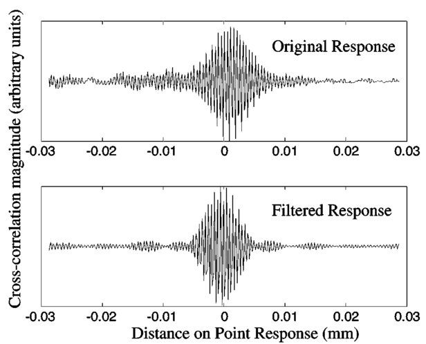

The second example image is of rat mammary tissue. Figure 3 shows the power spectral density of the source S˜₀(ν) (solid line) and of the corrected instrument response L˜₀(ν) (dashed line). Again, the effect of the filtering is to smooth the instrument response. This effect is seen more clearly in Fig. 4, which is the numerically estimated point responses of the original spectrum (solid line) and of the filtered instrument response (dashed line). The sidelobes of the response magnitude (shown in logarithmic scale) of the filtered response decrease much faster than the uncorrected spectrum. Because of the presence of the sidelobes in the source spectrum point response, the rms width of the response is 14.3 μm as opposed to 3.3 μm for the filtered response. However, the magnitude of the RMS width can overstate the improvement because the rms width is very sensitive to sidelobes further from the center of the point response. We note that reducing the rms width of the point spread response may increase the magnitude of the sidelobes near the center of the response when the peripheral sidelobes are reduced, because the goal is to reduce the overall rms width of the point response, and not eliminate any specific sidelobe feature.

Figure 3

Spectrum of source (solid line) and sidelobe-corrected instrument response function (dashed line). The OCT system used a UHNA3 fiber as a source, and spectra were obtained from scattering off of the rat mammary tissue.

Figure 4

Magnitude of the estimated point response of the source spectrum (solid line) and sidelobe-corrected point response function (dashed line). Plots correspond to spectra shown in Fig. 3.

Figure 5 shows the two images of the rat mammary tissue without (top) and with (bottom) sidelobe suppression. The reconstruction was achieved using the steps outlined in Table 1. Macroscopically, these images, which are plotted on a linear amplitude scale rather than a logarithmic scale, look very similar because the modifications to the image occurs at the smallest scales. Linear data scales were used because the data shown are more like the interference signal directly sampled and quantized by the detection electronics. To see the improvement, the three boxed sections of the image of Fig. 5 are shown in Fig. 6. The effect of the sidelobe suppression filter is to make the images of point-like objects smaller and sharpen the boundaries. The improvement may help to distinguish small pointlike scatterers in tissues such as cellular organelles, where a sidelobe might be mistaken for a separate structure. Using Eq. (10), the signal-to-noise ratio of the uncorrected image of Fig. 5 was calculated to be 30.75, and the sidelobe corrected image SNR was 57.20. The increase of SNR over the case without any filtering can be attributed to the exclusion of noise in frequency bands where there is little available signal.

Figure 5

Uncorrected (top) and corrected (bottom) images of rat mammary tissue. Image sizes are 1.5×0.5 mm.

Figure 6

High-magnification comparison of boxed areas from Fig. 5 between uncorrected (top) and corrected (bottom) images. For scale, the region in A is 70×70 μm.

Table 1

Procedure for utilizing sidelobe suppression method.
1. Measure the axial scan data cross-spectral density and compute the Fourier transform W˜(ν) of each axial scan.
2. Average \|W˜(ν)\|² of all of the axial scans together to produce an estimate of the signal power spectral density W˜₀(ν)²=S˜₀(ν)²G˜₀(ν)²+N˜₀(ν)².
3. Assuming the noise power spectral density is constant, average together the power spectral density of a frequency band known not to be emitted by the laser source to estimate the noise power spectral density.
4. Subtract the noise power spectral density estimate N˜₀(ν)² from the estimated W˜₀(ν)² to find an estimate of S˜₀(ν)², assuming that G˜₀(ν)²=1. Set any negative S˜₀(ν)² to zero.
5. Use Eq. (12) to compute α₀, and then select α=kα₀, where k is a predetermined constant on the order of unity that provides the desired tradeoff between resolution and noise. Select β∝1/α to aid convergence.
6. Use Eq. (11) to iteratively compute L˜(ν) starting with the Weiner filter.
7. Compute H˜(ν)=L˜(ν)/S˜₀(ν).
8. Compute the estimate of G˜(ν)=H˜(ν)W˜(ν) for each axial scan.

We note that achieving benefit from this method is contingent on obtaining an accurate estimate of the power spectral density of the source and the noise. In addition, the stability of the interferometer is of paramount importance because small random path-length variations, caused by vibrations or thermal fluctuations for example, will alter the spatial frequencies of the interferogram sufficiently to cause significant error in the Fourier analysis of the interferogram. For this reason, special attention must be paid to eliminating these fluctuations to utilize this method successfully.

The method presented provides a means to balance noise suppression and sidelobe suppression by iteratively computing an optimal filter. Two key advantages are gained, a filter best suited to the particular instrument is found, and the computational cost of obtaining this filter need be paid only once so long as the input spectrum remains unchanged. Alternatively, if the source spectrum is inconsistent, but remains stable during the acquisition of a single image, then the method can be adapted to provide a new filter for each image if the spectrum is measured or estimated for each image, hence it is dynamically “adaptive” to the source. In light of this work, achieving a broad, stable spectrum should be more important than achieving a Gaussian spectrum because digital correction can be applied to the data. The method fails to achieve desirable results in certain circumstances where the linearity of the data acquisition is compromised: if clipping occurs in the electronic amplifier before sampling, if the signal is digitized with low accuracy, or if the dispersion of the intervening medium is uncompensated. Methods, such as the one presented here, implemented by digital signal processing, will produce a more flexible instrument able to tolerate spectral nonuniformity without degrading performance.

Acknowledgments

We thank Keith Singletary from the Division of Nutritional Sciences and the Department of Animal Sciences and Wei Luo from the Beckman Institute for their assistance in animal care and handling for this research. Funding for this research was provided by the National Science Foundation (BES-0086696), the Whitaker Foundation, joint support from the National Aeronautics and Space Administration and the National Cancer Institute (NAS2-02057), and the National Institutes of Health (1 RO1 EB00108-1).

REFERENCES

1.

W. Drexler , U. Morgner , F. X. Kartner , C. Pitris , S. A. Boppart , X. Li , E. P. Ippen , and J. G. Fujimoto , “In vivo ultrahigh resolution optical coherence tomography,” Opt. Lett. , 24 1221 –1223 (1999). Google Scholar

2.

B. Povazay , K. Bizheva , A. Unterhuber , B. Hermann , H. Sattmann , A. F. Fercher , W. Drexler , W. Apolonski , W. J. Wadsworth , J. C. Knight , P. St. J. Russell , M. Vetterlein , and E. Scherzer , “Submicrometer axial resolution optical coherence tomography,” Opt. Lett. , 27 1800 –1802 (2002). Google Scholar

3.

S. Coen , A. H. L. Chau , R. Leonhardt , J. D. Harvey , J. C. Knight , W. J. Wadsworth , and P. S. J. Russell , “Supercontinuum generation by stimulated Raman scattering and parametric four-wave mixing in photonic crystal fibers,” J. Opt. Soc. Am. B , 19 753 –764 (2002). Google Scholar

4.

J. M. Dudley , L. Provino , N. Grossard , H. Maillote , R. S. Windeler , B. J. Eggleton , and S. Coen , “Supercontinuum generation in air-silica microstructure fibers with nanosecond and femtosecond pulse pumping,” J. Opt. Soc. Am. B , 19 765 –771 (2002). Google Scholar

5.

S. Coen , A. H. L. Chau , R. Leonhardt , J. D. Harvey , J. C. Knight , W. J. Wadsworth , and P. S. J. Russell , “White-light supercontinuum generation with 60-ps pump pulses in a photonic crystal fiber,” Opt. Lett. , 26 1356 –1358 (2001). Google Scholar

6.

I. Hartl , X. D. Li , C. Chudoba , T. H. Ko , J. G. Fujimoto , J. K. Ranka , and R. S. Windeler , “Ultrahigh-resolution optical coherence tomography using continuum generation in an air silica microstructure optical fiber,” Opt. Lett. , 26 608 –610 (2001). Google Scholar

7.

T. A. Birks , W. J. Wadsworth , and P. S. J. Russell , “Supercontinuum generation in tapered fibers,” Opt. Lett. , 25 1415 –1417 (2000). Google Scholar

8.

D. L. Marks , A. L. Oldenburg , J. J. Reynolds , and S. A. Boppart , “Study of an ultrahigh numerical aperture fiber continuum generation source for optical coherence tomography,” Opt. Lett. , 27 2010 –2012 (2002). Google Scholar

9.

G. E. Backus and F. Gilbert , “The resolving power of gross Earth data,” Geophys. J. R. Astr. Soc., 16 169 –205 (1968). Google Scholar

10.

G. E. Backus and F. Gilbert , “Uniqueness in the inversion of inaccurate gross Earth data,” Philos. Trans. R. Soc. London , 266 123 –192 (1970). Google Scholar

11.

A. W. Schaefer , J. J. Reynolds , D. L. Marks , and S. A. Boppart , “Real-time digital signal processing-based optical coherence tomography and Doppler optical coherence tomography,” IEEE Trans. Biomed. Eng. , 51 186 –190 (2003). Google Scholar

12.

J. M. Schmitt , “Restoration of optical coherence images of living tissue using the CLEAN algorithm,” J. Biomed. Opt. , 3 66 –75 (1998). Google Scholar

13.

D. Piao, Q. Zhu, N. K. Dutta, S. Yan, and L. L. Otis, “Coherent artifacts in optical coherence tomography: observation and cancellation,” Proc. IEEE 27th Annual NE Bioengineering Conf. 2001, pp. 53–54 (2001).

14.

Y. Zhang , M. Sato , and N. Tanno , “Resolution improvement in optical coherence tomography by optimal synthesis of light emiting diodes,” Opt. Lett. , 26 205 –207 (2001). Google Scholar

15.

Y. Zhang , M. Sato , and N. Tanno , “Numerical investigations of optimal synthesis of several low coherence sources for resolution improvement,” Opt. Commun. , 192 183 –192 (2001). Google Scholar

16.

Y. Zhang , M. Sato , and N. Tanno , “Resolution improvement in optical coherence tomography based on destructive interference,” Opt. Commun. , 187 65 –70 (2001). Google Scholar

17.

R. Tripathi , N. Nassif , J. S. Nelson , B. H. Park , and J. F. de Boer , “Spectral shaping for non-Gaussian source spectra in optical coherence tomography,” Opt. Lett. , 27 406 –408 (2002). Google Scholar

18.

J. F. de Boer , C. E. Saxer , and J. S. Nelson , “Stable carrier generation and phase-resolved digital data processing in optical coherence tomography,” Appl. Opt. , 40 5787 –5790 (2001). Google Scholar

19.

E. D. J. Smith , S. C. Moore , N. Wada , W. Chujo , and D. D. Sampson , “Spectral domain interferometry for OCDR using non-Gaussian broad-band sources,” IEEE Photonics Technol. Lett. , 13 64 –66 (2001). Google Scholar

20.

E. D. J. Smith , N. Wada , W. Chujo , and D. D. Sampson , “High resolution OCDR using 1.55 μm supercontinuum source and quadrature spectral detection,” Electron. Lett. , 37 1305 –1307 (2001). Google Scholar

21.

M. D. Kulkarni , C. W. Thomas , and J. A. Izatt , “Image enhancement in optical coherence tomography using deconvolution,” Electron. Lett. , 33 1365 –1367 (1997). Google Scholar

22.

D. L. Marks , A. L. Oldenburg , J. J. Reynolds , and S. A. Boppart , “A digital algorithm for dispersion correction in optical coherence tomography for homogeneous and stratified media,” Appl. Opt. , 42 204 –217 (2003). Google Scholar

23.

T. Asakura and T. Ueno , “Apodization for minimizing the second moment of the intensity distribution in the Fraunhofer diffraction pattern,” Nouv. Rev. Opt. , 7 199 –203 (1976). Google Scholar

24.

G. Gbur and P. S. Carney , “Convergence criteria and optimization techniques for beam moments,” Pure Appl. Opt. , 7 1221 –1230 (1998). Google Scholar

Notes

Address all correspondence to Daniel Marks and Stephen Boppart, Univ. of Illinois/Urbana-Champaign, Beckman Institute, 405 N. Mathews, Urbana, IL 61801. Tel: 217-244-2494; Fax: 217-244-6898; E-mail: dmarks@uiuc.edu, boppart@uiuc.edu

Citation Download Citation

Daniel L. Marks, Paul Scott Carney, and Stephen A. Boppart M.D. "Adaptive spectral apodization for sidelobe reduction in optical coherence tomography images," Journal of Biomedical Optics 9(6), (1 November 2004). https://doi.org/10.1117/1.1806471

Published: 1 November 2004

Access the abstract

JOURNAL ARTICLE
7 PAGES

DOWNLOAD PAPER SAVE TO MY LIBRARY

GET CITATION

CITATIONS

Cited by 13 scholarly publications and 5 patents.

Explore citations on Lens.org

RIGHTS & PERMISSIONS

Get copyright permission Get copyright permission on Copyright Marketplace

KEYWORDS

Optical coherence tomography

Signal to noise ratio

Optical filters

Filtering (signal processing)

Optical fibers

Apodization

Digital filtering

1.

Introduction

2.

Derivation