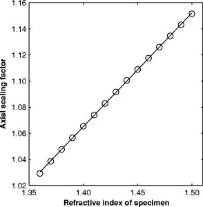
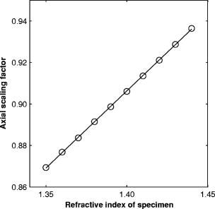
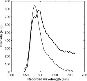
1.

Introduction

Refractive index of biological tissue is a basic material parameter that characterizes how light interacts with biological tissue. Scattering of tissue is characterized by microscopic fluctuations in the refractive index,^{1, 2} while the concept of macro refractive index, or average refractive index on a macroscopic scale, is relevant in problems such as light propagation at the interface between water and tissue, between two tissue types, or between tissue and an optical detector such as an optical fiber. When distances are measured using optical techniques, the optical path length defined as the real path length multiplied by the refractive index of the medium in which the light is propagating is obtained. When we want to measure real (physical) distances, the refractive index has to be known accurately. In optical tomography, for instance, 3-D reconstructions of tissue are obtained from time of flight measurements of photons: the time depends on the physical distance, on the diffusion of the medium, and on the refractive index of the medium. In confocal microscopy, 3-D measurements of small objects can be made, but the distances measured also need to be scaled by the refractive index of the tissue.

Because most types of tissue are highly diffuse, inhomogeneous, and optically turbid, traditional methods for determining the refractive index of fluids and solids are difficult to apply. Specifically, a basic problem in using traditional methods such as refractometers is to assure perfect optical contact between the tissue and the optical elements over a large zone. In many optical studies, crude estimates of refractive index of tissue are used, based on the fact that the main constituent of tissue is (salt) water-filled cells. Precise experimental determination of refractive index of tissues under study is most often not done, and for many kinds of tissue the index of refraction is not listed in literature.³ The index of refraction of tissue is an important optical constant, but values used are often without experimental basis.

A limited number of attempts have been made to determine the refractive index of biological tissue with good accuracy. Bolin ⁴ proposed a method where the cladding of an optical fiber is replaced by tissue, and the angle of the cone of light emerging from the fiber is measured. They measured refractive index in different types of tissue. For bovine striated muscle, they found $n=1.412$ for a wavelength of $632.8\mathrm{nm}$ , with an intersample standard deviation of 0.006. For bovine adipose, a value of $n=1.455$ , without specification of standard deviation, is given.

Tearney ⁵ proposed the use of optical coherence tomography. They measured refractive index of several types of human tissue in vitro and in vivo. For cardiac muscle, a value of $n=1.382\pm 0.007$ was found using a wavelength of $1300\mathrm{nm}$ . For human adipose tissue, the value was $n=1.467\pm 0.008$ . The method was demonstrated on $500\text{-}\mu \mathrm{m}$ -thick samples.

Li and Xie⁶ devised a method based on total internal reflection using a laser beam of diameter $0.1\mathrm{mm}$ and a semicylindrical lens in contact with the tissue specimen. The authors used the method to measure refractive index of human blood and porcine muscle. At a wavelength of $632.8\mathrm{nm}$ , a refractive index of $1.380\pm 0.007$ and $1.460\pm 0.008$ was found in two muscle samples.

Tsenova and Stoykova⁷ used a laser refractometer to measure the refractive index of dehydrated, thin tissue samples. To obtain values for fresh tissue, they multiply values with a crude estimate of the water content, and give a general value of 1.4 for refractive index of tissue.

We propose a new and straightforward method for determining the refractive index of tissue with high accuracy, using a confocal microscope. In a previous work, we demonstrated how accurate thickness data are obtained from confocal microscope virtual sections.⁸ The method takes into account the 3-D point spread function (PSF) of the microscope, and we showed that thickness of polymer films (of known refractive index) could be measured with an accuracy better than 0.5%. We now show how this method may be adapted to determine the refractive index of thin tissue layers.

2.

Theory

In confocal laser scanning fluorescence microscopy, a thin specimen is positioned in the lateral $(x,y)$ plane of the specimen table, and the objective lens focuses the light of the illuminating laser to a spot at a certain depth $z$ within the specimen. The fluorescence light emitted by that point within the object is imaged by the objective lens. By using a pinhole positioned in the focal point of the imaging optics, only the light coming from a single point in space is being recorded, at least in the approximation of geometric optics. Depending on the type of confocal microscope used, the pinhole can be positioned at different locations of the imaging pathway. In the microscope we used, the pinhole is positioned just before the detector. Due to the wave character of light and due to the finite size of the pinhole, we record not only the light coming from a single point, but light emitted from within a small 3-D volume element (described by the PSF of the instrument). Hence, the borders of an object along its height direction are not seen as clear cut edges, but rather as slightly blurred transients in intensity, which are the convolution of the step response of the object with the PSF of the microscope. Due to absorption and scattering, the recorded intensity also diminishes with focusing depth, putting a limit to the thickness of specimens that can be imaged.

Virtual sections through the specimen are obtained by scanning along the $x$ or $y$ direction, and along the $z$ direction, and measuring the intensity of the fluorescence light emitted by each point of the object. To obtain the highest possible resolution, immersion-type objective lenses are used, and a droplet of immersion fluid (usually water or oil) is put between the front of the objective lens and the cover slip, which rests on the object. In confocal microscopy, distances measured along the $z$ axis are optical path lengths. If a refractive index mismatch exists between the immersion medium of the objective lens and the refractive index of the specimen, this mismatch causes a scaling factor between measured thickness and actual physical thickness of the specimen.

Figure 1 shows how the objective lens of a microscope focuses light through an immersion medium with refractive index $n_1$ into a specimen with refractive index $n_2$ . If the specimen and the immersion medium have the same refractive index, the light rays follow a straight path and are focused at a nominal focus position (NFP). In case of a mismatch, however, the light path is broken at the interface, and rays are focused at an actual focus position (AFP), which is different from the NFP. In Fig. 1, we show the case where $n_1<n_2$ : the full lines depict the light rays in case of matched media, and the dashed lines show the real light path. The difference in distance between the location of the AFP and the NFP is known as “focal shift.”

Fig. 1

Basic scheme of an immersion objective lens that focuses to a point in a specimen that has a higher index of refraction than the immersion medium. The focus is not located in the NFP, but is shifted to a deeper AFP. The difference of the AFP and the NFP is called the focal shift. When focusing to a deeper position (right side of the figure), the focal shift increases. When moving the objective lens over a distance $\Delta Z$ , the AFP moves over a distance $\Delta Z^{\prime }$ , making objects appear thinner than they are. The ratio $\Delta Z^{\prime }∕\Delta Z$ is called the axial scaling factor.

If we now focus on a deeper location in the object, as shown in the right-hand side of Fig. 1, the distance between AFP and NFP changes: in the case of $n_1<n_2$ , the focal shift increases with object depth. When the objective lens is moved over a distance $\Delta Z$ to focus on a point deeper in the object, the reading of the $z$ -translation stage shows the value of the NFP, which also moves over the distance $\Delta Z$ . In reality though, the light is coming from the AFP, which has moved down over a larger distance $\Delta Z^{\prime }$ . To first focus on the top border of the object and then on the bottom, the objective lens is moved over a smaller distance along the $z$ axis than the thickness of the object. If a virtual section through the object is recorded (by scanning along the $x$ and $z$ axis), this section will appear thinner than the actual physical thickness of the object. The ratio $\Delta Z^{\prime }∕\Delta Z$ , and hence the ratio of the real and the measured object thickness, is known as the axial scaling factor (ASF).

Assuming simple geometric optics and paraxial light rays, it can easily be seen that the ASF can be approximated as the ratio of the refractive indices. If one wants to obtain actual thickness data from virtual slices recorded with the confocal microscope, one needs to scale the measured $z$ values by multiplying with the ASF. To be able to do so, one needs to know the refractive index of the immersion fluid and the specimen. If, however, one knows the exact physical thickness of the specimen, one can use the ASF the other way around, and calculate the index of refraction of the object, since the index of refraction of the immersion fluid is of course a known constant.

The problem is now to determine the actual physical thickness of the specimen. For technical objects such as plastic foils, one can use alternative methods such as mechanical sensors, but these are of no use for soft biological material. We therefore need to determine the thickness in a noncontacting, optical way. The trick we use is to put the specimen next to a layer of immersion fluid of exactly the same physical thickness. This situation can easily be obtained by putting the specimen on a support glass, next to a droplet of immersion fluid, and then sandwich both specimen and fluid under a cover glass. As the cover glass rests on the specimen, the layer of fluid next to the specimen has exactly the same thickness. Because this fluid has the same index of refraction as the immersion fluid, no axial scaling effects will take place: in the fluid layer, AFP and NFP coincide and the physical thickness of the layer is the same as the optical thickness measured on a virtual section image. This thickness is equal to the physical thickness of the specimen, and hence we can readily calculate the specimen refractive index using the ASF and the known refractive index of the immersion fluid.

In reality, however, the situation is more complicated. Due to the wave nature of light, the focal point takes the shape of a 3-D volume, known as the PSF. From vectorial diffraction theory, it can be shown that this volume also changes shape with increasing focus depth. If an accuracy of only a few percent is needed, the paraxial approximation of the ASF can be used; but to make very accurate measurements, the PSF needs to be taken into account.

The ASF as a function of increasing object depth can be calculated using the PSFs of the confocal microscope at increasing focusing depths. Because confocal imaging is a two-step process (i.e., illumination of the specimen by a point source and detection of the emitted light of the specimen by a point detector that is placed symmetrically to the point source), the product of the illumination PSF and detection PSF results in the confocal PSF (Hell and Stelzer⁹). We have calculated the illumination and detection PSF with the theoretical model suggested by Hell ¹⁰ It is based on vectorial diffraction theory using the Huygens-Fresnel principle and Fermat’s principle. We used the same calculation procedure as Hell, but we refined it by taking into account the shape of the illumination profile at the exit pupil of the objective lens when calculating the illumination PSF. Hell assumed a homogeneous entrance profile, while we used the actual, truncated-Gaussian illumination profile (Kuypers, Dirckx, and Decraemer¹¹).

The confocal PSF is given by a 3-D intensity distribution $I_{\mathrm{NFP}}(x,y,z)$ and describes how the detected image of a point-like object at a given NFP is blurred in space. The plane spread function or $z$ response describes how a horizontal plane is blurred. Because we are interested in the axial response of a horizontal layer, $z$ responses for different depths were calculated as:

In another paper, we used this calculation to take the PSF into account when calculating the ASF (Kuypers ⁸), and we used these corrected ASFs to calculate the thickness of objects with known refractive index and known physical thickness. For those measurements, thin polymer films were prepared, and their physical thickness was measured with a scanning electron microscope. The scaling factor obtained from the model agreed very well with measured ratios of actual and measured thickness, in cases of index mismatch both larger and smaller than unity.

As explained with the paraxial approximation, we can now use this method the other way around to determine the unknown index of refraction of an object by determining its physical thickness from a measurement on an adjacent layer of fluid with known refractive index. We use the Kuypers model⁸ to calculate the specimen refractive index from the measured ASF, in the case of water (Fig. 2 ) and of oil (Fig. 3 ) as immersion mediums. We performed the calculations for a typical water immersion objective lens with a numerical aperture (NA) of 1.2, and a typical oil immersion lens with NA of 1.3. The circles in Figs. 2 and 3 indicate calculated values: due to the nonlinear nature of the PSF, there is a small deviation from linearity, i.e., from the solid line that represents the best straight line through the data. In the first order, however, the PSF correction leads to a linear correction on the ASF. If the actual axial scaling factor (ASF) is determined experimentally, as the ratio of measured object thickness and actual physical object thickness, the model can now be used to calculate the corresponding index of refraction of the object. As the deviation from linearity is extremely small, we can use the straight line fit of Figs. 2 and 3 and calculate the refractive index by linear interpolation:

Fig. 2

Axial scaling factor as a function of the refractive index of the specimen in case of water immersion. The circles indicate values calculated with our model for an objective lens of 1.2 NA, and the solid line shows the best linear fit through the data.

Fig. 3

Axial scaling factor as a function of the refractive index of the specimen in case of oil immersion. The circles indicate values calculated with our model for an objective lens of 1.3 NA, and the solid line shows the best linear fit through the data.

3.

Method

3.1.

Specimen Preparation

To demonstrate our method, we chose bovine muscle tissue, because for this type of tissue good reference data are available for comparison.⁴ We took two pieces about $0.5\times 0.5\times 1\mathrm{cm}$ out of the same muscle, one perpendicular to the muscle fibers and one parallel to the fibers. The samples were frozen using standard histologic techniques by submerging them in 2-methylbutane (for good thermal conductance) at fluid nitrogen temperature. This ultra-fast freezing process assures that no tissue swelling occurs and that cells remain intact. Next, the specimens were transferred to a freezing microtome $(-20°\mathrm{C})$ where slices of different thicknesses, ranging between 30 and $100\mu \mathrm{m}$ , were cut. The slices of about $5\times 5\mathrm{mm}$ were spread out on a microscope glass and a droplet of immersion fluid was put next to the specimen. In the case of water, the immersion fluid was dyed with rhodamine B to obtain fluorescence. In the case of oil, no dye was needed to obtain a signal. In both cases, the tissue itself could remain completely untreated, as it showed sufficient autofluorescence under the microscope. A cover glass was then put onto the tissue in a tilting motion, so that surplus fluid was pushed away without entering between the contact surface of the tissue and the cover glass. In this way, we obtained a sandwich preparation comprised of a layer of tissue next to a layer of fluid of exactly the same thickness, between two thin, plan-parallel layers of glass. The preparation was then put in the microscope with a droplet of immersion fluid (water or oil, same fluid as within the preparation) between the cover slip and the objective lens.

Figure 4 shows how the specimen and fluid layer are mounted. The figure is not to scale: in reality the specimen is extremely thin. In our case, we used an invert confocal microscope, so the objective lens is located beneath the specimen. We schematically represent the two adjacent layers of tissue (gray) and immersion fluid (dotted), which are of equal thickness.

Fig. 4

Diagram of the measurement arrangement. A layer of tissue and immersion fluid are sandwiched between a microscope glass and a cover glass. The invert confocal microscope objective lens is positioned beneath the object. By scanning along the $x$ axis at subsequent depth locations and recording the emitted light at each object point in the $x\text{-}z$ plane, a virtual slice image is obtained.

We made a total of 14 preparations, 7 with oil and 7 with water. For each immersion fluid, four preparations were made with muscle slices cut in parallel and three in a direction orthogonal with respect to the muscle fibers.

3.2.

Measurement Method

For each preparation, 9 to 10 virtual section images were recorded, each containing the interface between tissue and fluid (Figs. 5 and 6 ). We used the Zeiss Lsm 410 invert confocal fluorescence microscope with a $1.2\mathrm{NA}$ water immersion objective lens (C-Apochromat $40\times$ , with correction collar) or a 1.3 oil immersion objective lens (Plan-Apochromat $40\times$ ), and an excitation wavelength of $488\mathrm{nm}$ . A low-pass filter was positioned before the detector, so that fluorescence light was measured with wavelengths longer than $510\mathrm{nm}$ . With these parameters, the axial resolution of the microscope is about $0.8\mu \mathrm{m}$ , so we used a standard factory setting for the scanning step in $z$ direction of $0.625\mu \mathrm{m}$ .

Fig. 5

(a) Virtual section of a slice of bovine muscle tissue next to a layer of water, measured with a water immersion objective lens. The muscle shows strong autofluorescence, and the water was slightly stained with rhodamine B. The thicknesses are indicated by the white bars. Both layers have equal physical thickness, but due to refractive index mismatch, the tissue layer appears thinner. (b) Intensity profiles along the $z$ position through the virtual section shown in (a), through the muscle tissue (left) and the water layer (right). The thickness obtained by the eye is indicated by the vertical line. The thickness obtained as the difference in $z$ position of the calculated positions (asterisk) is practically equal.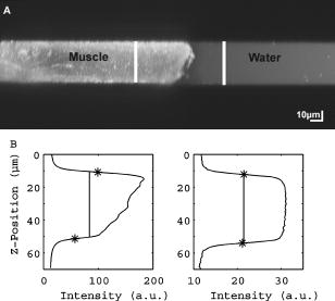

Fig. 6

(a) Virtual section of a slice of bovine muscle tissue next to a layer of oil, measured with an oil immersion objective lens. The oil shows stronger autofluorescence than the tissue. The thicknesses are indicated by the white bars. Again, both layers have equal physical thickness, but due to refractive index mismatch, the tissue layer appears significantly thicker. (b) Intensity profiles along the $z$ position through the virtual section shown in (a), through the muscle tissue (left) and the oil layer (right). The thickness obtained by the eye is indicated by the vertical line. The thickness obtained as the difference in $z$ position of the calculated positions (asterisk) is practically equal.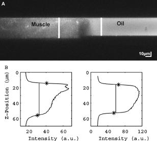

To measure the thickness at one location on the object, the objective lens is moved along the $z$ direction by a stepper motor, and the intensity of the fluorescence light obtained at each depth is recorded. Due to the pinhole in a focal point in the imaging pathway, only light emitted from one single point in space (or in reality from the PSF volume) is recorded. To record a virtual section, the specimen is scanned along the $x$ direction. Such scanning could be done using a second stepper motor to translate the specimen table, but in the Zeiss Lsm 410 (as in most confocal microscopes), scanning along the $x$ or $y$ direction is performed by tilting mirrors positioned in the beam delivery pathway, while the object and objective lens remain in the same position. Because the tilting mirrors can move much faster than the $z$ -translation stage, virtual sections are recorded line by line along the $x$ axis, each line at a next depth step. The step size along the $x$ and $z$ direction is chosen according to the resolution of the instrument settings. The tilting mirrors allow us to scan a region $320\mu \mathrm{m}$ wide when using an objective lens with a magnification of 40. To obtain thickness data over larger object zones, the object table is moved in the $x$ or $y$ direction.

The optical thickness of the adjacent fluid and tissue layers in the section images [i.e., Figs. 5(a) and 6(a)] have to be precisely measured. This can be done simply by judging by the eye (e.g., on a zoomed-in image on a computer screen) where the object starts and ends, or one can make a plot of the intensity profile along the $z$ axis at a given location on the section. In another paper,⁸ we used dyed plastic foils of calibrated thickness and showed that the front and back of the specimen coincide to a very good precision with the location of a minimum in the second derivative of the intensity profile. However, in specimens where the transients in intensity are clearly seen, judging by eye where the front and back plane of the object is situated, yields the same thickness values to a very good accuracy, without the need of supplementary analysis. In Figs. 5(b) and 6(b), we show the intensity profile through the virtual sections (averaged over $20\mu \mathrm{m}$ along the lateral axis) of the muscle tissue (left) and the immersion fluid layer (right). The thickness obtained by eye (vertical line) and the thickness obtained as the difference of the calculated positions (asterisk) is practically equal.

First, the thickness of the fluid layer is determined. Since the fluid in the preparation has the same refractive index as the immersion medium, there is no refractive index mismatch. Therefore, the actual thickness of the fluid layer is immediately obtained by multiplying the number of depth pixels with the calibration factor of $0.625\mu \mathrm{m}\text{per}\text{pixel}$ .

As the specimen thickness exactly equals the thickness of the fluid layer, we now also know the actual physical thickness of the specimen. Next, we measure the optical thickness of the tissue specimen next to the fluid layer. The axial scaling factor is calculated as the ratio of the physical thickness and the measured thickness. Using Eq. 3 or 4, we then can calculate the refractive index of the specimen.

4.

Results

In Fig. 5(a), we showed a virtual section through a sample of bovine muscle and water. Tissue and water layers have exactly the same physical thickness, yet in the image the muscle appears thinner than the water layer. It is exactly this difference in optical thickness that contains the information about the refractive index. Because we wanted to maximally reduce any change in tissue properties, only an extremely small amount of dye was used to make the water layer fluoresce, so that no staining of the tissue occurs. The tissue itself looks brighter due to strong autofluorescence. Figure 6(a) shows a section through a muscle/oil interface. No staining of the oil was necessary, as it even shows stronger autofluorescence than the tissue. We clearly see that the measured thickness of the muscle is now considerably larger than the measured thickness of the oil layer, due to the rather large difference in refractive index.

For the water preparation, we recorded a total of 36 virtual sections on the parallel cut specimens, and on each of them we determined the thickness of the tissue sample and of the water layer. We found an average axial scaling factor of $1.0490\pm 0.0013$ . On the three specimens cut at right angles with the muscle fibers, we recorded a total of 29 virtual sections, and found a mean axial scaling factor of $1.0484\pm 0.0022$ . Averaged over all measurements, an axial scaling factor of $1.0487\pm 0.0012$ is found. The precision on these data was obtained as the standard deviation calculated on the average. Using Eq. 3 and the rules of error propagation, we finally calculated the refractive index of bovine muscle tissue and its measuring precision: $n=1.381\pm 0.003$ .

In the same way, a mean axial scaling factor of $0.8943\pm 0.0016$ was determined from the oil preparation. Using Eq. 4 for the oil preparations, we obtained a refractive index for the bovine muscle of $n=1.384\pm 0.004$ .

As refractive index is known to be a function of the wavelength, it is necessary to know the spectrum of the fluorescence light used to obtain the images. We measured the fluorescence spectrum obtained behind the low-pass filter used in the microscope, using a grating spectrometer (Specbos 100, Jeti Inc., Jena, Germany). Figure 7 shows the spectra of rhodamine B dissolved in water (thin line) and of bovine muscle tissue (thick line). The full width of the curves at half of the maximal intensity is a common measure to estimate the bandwidth of the light used for imaging. At half of maximal intensity, the fluorescence light obtained from muscle varies from $560\text{to}640\mathrm{nm}$ and has a maximum at $592\mathrm{nm}$ . The fluorescence bandwidth of rhodamine B is about half as large and has a maximum at $582\mathrm{nm}$ .

Fig. 7

Fluorescence spectra of rhodamine B (thin line) and bovine muscle tissue (thick line). The peak intensity for rhodamine B is located at $582\mathrm{nm}$ , while the tissue shows peak fluorescence intensity at a slightly larger wavelength of $592\mathrm{nm}$ .

5.

Discussion

6.

Conclusions

We develop a new method to measure the refractive index of tissue with high accuracy. The method is simple to use and can be performed on any confocal microscope. Thanks to the method that we developed earlier to take the PSF of the microscope into account, we can calculate the physical specimen thickness from the measured thickness with high accuracy. Using this technique, we are able to present highly accurate values of the index of refraction of bovine muscle tissue. For specimens cut at right angles with the muscle fibers and parallel with the fibers, we obtain slightly different values for the index of refraction, but within the measuring precision the values overlap. As a final result, we find that the index of refraction of bovine muscle tissue is given by

As shown by other authors,^{4, 6} values can differ significantly between individual specimens and between different locations within one specimen. Our technique can easily be implemented using any confocal microscope, and therefore allows us to determine the index of refraction of the specific type of tissue and species that is used in an optical experiment, rather than using standard values. The method we present here, which only needs thin specimens, becomes essential when only small tissue samples are available and when measuring, e.g., the index of refraction of thin membranes such as the eardrum¹² or the cerebral membrane. Together with a diffusion coefficient, refractive index is one of the basic parameters needed to perform quantitative optical measurements, e.g., optical tomography through the exposed cerebral membrane. In research on the mechanics of hearing, thickness distribution of the eardrum is an essential parameter to developing highly accurate finite element models of the middle ear, which are a key element in understanding the complex mechanical behavior of the ear. Thickness distributions along sections through the eardrum can be measured using the confocal microscope if the refractive index of the tissue is known.¹²