1.

Introduction and Motivation

With the routine achievement of single molecule sensitivity in fluorescence microscopy, fluorescence correlation spectroscopy (FCS) and related fluctuation spectroscopy methods such as distribution analysis are becoming increasingly important research tools in biophysical and biomedical research.^{1, 2, 3, 4, 5, 6, 7, 8} These methods are able to characterize the chemical and physical dynamics of biological systems, including the capability to measure the hydrodynamic mobility, interactions, and chemical kinetics of biomolecules in solution and within living cells. Fluctuation spectroscopy measurements are typically performed using either two-photon or one-photon confocal microscopy to achieve a well defined finite fluorescence observation volume in three dimensions.^{9, 10, 11, 12} Information recovery from fluctuation spectroscopy measurements requires both correct physical models for the underlying fluctuation dynamics and an accurate representation of the size and profile of the fluorescence observation volume. The 3-D Gaussian (3-DG) spatial profile is the most commonly used representation of the fluorescence observation volume in both one- and two-photon FCS measurements. While not an exact representation of true observation volume profile, under appropriate experimental conditions the 3-DG model can be used with good success in analyzing fluctuation spectroscopy data.^{10, 13} On the other hand, it is not widely recognized that the photophysical dynamics of the fluorescence excitation process can lead to dramatic alterations in the size and shape of the observation volume. In particular, saturation of the fluorescence excitation can significantly increase the size and flatten the spatial profile of the observation volume, as is described in this work. When using focused laser excitation together with high numerical aperture lenses, these changes can become important even with relatively modest average excitation power. Moreover, saturation-modified observation volumes can be different for various fluorescent molecules, since the degree of saturation depends not only on the laser excitation but also the absorption cross section and excited-state lifetime of the fluorescent molecules in the sample. The lack of a quantitative characterization of the saturation-modified observation profiles not only has the potential to introduce systematic errors in FCS analysis, but also ultimately limits the flexibility of FCS applications, since any given set of measurements must be performed with fixed laser excitation to avoid altering the instrument calibration. It is therefore desirable to develop quantitative models for the saturation-modified volumes and corresponding fluctuation spectroscopy equations to facilitate accurate analysis and interpretation of FCS data over a wide range of measurement conditions. Quantitative models for the saturation modified profiles in two-photon microscopy have recently been published.¹⁴ We introduce a quantitative description of the modified volumes in one-photon confocal FCS measurements, and demonstrate their success in modeling the observed saturation-induced effects in measured one-photon FCS data. We begin with a review of the fluorescence measurement process, including a detailed discussion of how the observation volume is defined and characterized. We also include a brief discussion of basic FCS theory to highlight how the observation volume changes are important for one-photon FCS measurements. Finally, we introduce a simple curve fitting strategy based on modifications to the commonly used 3-DG FCS fitting functions and demonstrate that it can accurately account for the observed correlation curve amplitudes and relaxation times for experimental data acquired over a wide range of excitation conditions.

2.

Theory

2.1.

Fluorescence Excitation and Observation Volumes

The basic physics of fluorescence excitation is well understood.¹⁵ For continuous wave fluorescence excitation, the fluorescence signal emitted from a molecular population is linearly proportional to the steady-state fraction of molecules in the excited state $W\left(\mathbf{r}\right)$ , given by:

Eq. 1

$$W\left(\mathbf{r}\right)=\frac{1}{2}\frac{2w\left(\mathbf{r}\right)}{2w\left(\mathbf{r}\right)+\Gamma }.$$

Here $w\left(\mathbf{r}\right)$ is the space- and time-dependent absorption and stimulated emission rate, and $\Gamma$ denotes the spontaneous excited-state relaxation rate, which is inversely proportional to the fluorescence lifetime, as shown in Fig. 1 . For each molecule in the sample, the photon absorption rate is proportional to both its absorption cross section and the local excitation laser flux, and can be written as $w\left(\mathbf{r}\right)={\sigma }_1{I}_{0}S\left(\mathbf{r}\right)$ . Here ${\sigma }_1$ is the one-photon absorption cross section and $I_0$ represents the peak photon flux of the laser excitation. The distribution function $S\left(\mathbf{r}\right)$ describes the profile of the focused laser beam and accounts for the spatial variation of the molecular excitation rate. The peak intensity at the center of the beam (in $\text{photons}∕{\mathrm{cm}}^2∕\mathrm{s}$ ) is denoted $I_0$ , and for Gaussian beams can be determined in terms of the average power on the sample as $I_0=2⟨P⟩∕hv\pi {\omega }_0^2$ , where ${\omega }_0$ is the laser beam waist and $hv$ is the photon energy.

Fig. 1

A two-state model is sufficient to capture the important saturation dynamics. Here $w\left(\mathbf{r}\right)$ represents the local absorption and stimulated emission rates, and $\Gamma$ is the excited-state relaxation rate. The absorbed photons have energy $hv$ .

In confocal microscopy, the measured signal is limited by an emission pinhole that can be described in terms of a collection efficiency function $\Omega \left(\mathbf{r}\right)$ .⁹ Accounting for the local molecular concentration $C\left(\mathbf{r}\right)$ , the detected fluorescence signal per unit volume can be written as $\kappa C(\mathbf{r},t)W\left(\mathbf{r}\right)\Omega \left(\mathbf{r}\right)$ , where $\kappa$ is a constant that accounts for both the quantum yield and lifetime of the fluorophore, as well as the detection efficiency of the measurement system. The total measured fluorescence signal can be expressed by summing the fluorescence signal from all regions of the sample, and the total average measured fluorescence signal is written:

Eq. 2

$$⟨F⟩=\kappa \Gamma ⟨C⟩\int W\left(\mathbf{r}\right)\Omega \left(\mathbf{r}\right)d\mathbf{r}.$$

Formally, this spatial integral is evaluated over the full extent of the sample, although the physical region represented by the integration limits greatly exceeds the actual sample region that contributes significantly to the measured fluorescence signal. To estimate the size of the sample region from which most of the measured fluorescence signal is emitted, it is customary to define an observation volume as $V=\int \widehat{W}\left(\mathbf{r}\right)d\mathbf{r}$ .^{9, 16, 17} Here $\widehat{W}\left(\mathbf{r}\right)=W\left(\mathbf{r}\right)\Omega \left(\mathbf{r}\right)∕W\left(0\right)$ defines the profile of the observation volume. Formally, $\widehat{W}\left(\mathbf{r}\right)$ is a normalized distribution function that defines the relative probability of detecting fluorescence photons from molecules located in different regions of the sample, and the size of the measurement volume is computed with a spatial integral over this distribution function. It is the probabilistic nature of this volume definition that leads to changes in the calibrated measurement volume with excitation saturation, as is shown next. We note that although the computed volume provides a useful estimate for the size of the sample region from which the measured fluorescence signal originates, the actual measured signal is generated from a larger region of the sample than this computed volume implies.

Based on the definition for the observation volume, one can also introduce a molecular brightness parameter $\psi =\kappa \Gamma W\left(0\right)$ that specifies the average rate of fluorescence photon detection from molecules located at focal plane along the optical axis (i.e., in the center of the observation volume). The molecular brightness is a critical parameter in predicting the signal-to-noise ratio for fluctuation spectroscopy measurements, and also has important implications for measuring molecular interactions.^{18, 19} Using the volume and molecular brightness definitions together, the expression for the average measured fluorescence signal can be greatly simplified and expressed simply as:

Eq. 3

$$⟨F⟩=\psi ⟨C⟩V.$$

Since fluctuation spectroscopy analysis general involves computation of different fluctuation moments, the total volume defined before is not by itself sufficient to fully characterize the fluorescence observation volume. For FCS measurements, one must also characterize the spatial profile of the observation volume distribution function, which is quantified in terms of the $\gamma$ factor and is defined as:¹⁶

Eq. 4

$$\gamma =\frac{\int {\widehat{W}}^2\left(\mathbf{r}\right)d\mathbf{r}}{\int \widehat{W}\left(\mathbf{r}\right)d\mathbf{r}}.$$

The gamma factor has values between zero and unity, and specifies the steepness of the probabilistic boundaries that define the volume. Larger values correspond to sharper boundaries. A gamma value of unity, which is never achieved for optically defined observation volumes, corresponds to a uniform volume profile with sharp boundaries as in a physical container.

In the limit of low photon absorption rates relative to the spontaneous relaxation rate, i.e., when $w\left(\mathbf{r}\right)⪡\Gamma$ , Eq. 1 can be simplified as $W\left(\mathbf{r}\right)=w\left(\mathbf{r}\right)∕\Gamma$ . In this case, the molecular brightness can also be written simply as $\psi =\kappa {\sigma }_1{I}_0$ and the total fluorescence signal as well as the signal from any particular molecule has the familiar linear dependence on the excitation laser intensity. For this case, the volume integral can be simply represented as the integral of the normalized focused laser profile $S\left(\mathbf{r}\right)$ multiplied by the collection efficiency function, i.e., $\widehat{W}\left(\mathbf{r}\right)=S\left(\mathbf{r}\right)\Omega \left(\mathbf{r}\right)$ . As noted earlier, provided that certain optical conditions are met,¹³ a condition we assume for this work, this volume distribution function can be successfully approximated as a 3-D Gaussian distribution specified in cylindrical coordinates as:

Eq. 5

$${\widehat{W}}_{3\mathrm{DG}}\left(\mathbf{r}\right)={\widehat{W}}_{3\mathrm{DG}}(\rho ,z)=\exp (-2{\rho }^2∕{\omega }_0^2)\exp (-2z^2∕z_0^2),$$

where ${\omega }_0$ and $z_0$ are the $1∕e^2$ beam waists in the radial and axial directions, respectively. For this distribution, the volume can be computed analytically and is found to have the value $V_{3\mathrm{DG}}={(\pi ∕2)}^{3∕2}{\omega }_0^2{z}_0$ . The corresponding gamma factor value is ${\gamma }_{3\mathrm{DG}}=1∕2\sqrt{2}$ .

2.2.

Excitation Saturation

As shown before, in the limit of low excitation power, the excited-state population and fluorescence signal are linearly proportional to the excitation intensity. However, as the excitation power is increased to the point where the photon absorption rates are comparable to the spontaneous relaxation rate, the excited-state population will no longer increase proportionately with increases in the excitation intensity due to saturation. This characteristic behavior, specified by Eq. 1, is shown in Fig. 2 . The limit on the effective molecular excitation rate is due to both stimulated emission and the finite lifetime of the excited state. For a simple two-state system, at most, half of the molecules at any location within the focused laser excitation profile can occupy the excited state at any given time, as shown in the figure. Based on Eq. 1, it is relatively straightforward to write a more general expression for the molecular brightness that includes the saturation dynamics. Specifically,

Eq. 6

$$\psi =\frac{\kappa {\sigma }_1{I}_0}{1+I_0∕I_{\mathrm{sat}}}.$$

Here we have introduced a saturation intensity defined as $I_{\mathrm{sat}}=\Gamma ∕2{\sigma }_1$ . The saturation intensity corresponds to the excitation flux that would excite half of the molecules illuminated at that intensity if the linear relationship between the excited-state population and excitation flux were not limited by saturation dynamics. It is important to recognize that the saturation intensity depends not only on the laser flux but also on the absorption cross section and excited-state lifetime of the fluorophore. It is also useful to note that the saturation intensity does not depend on the diffusion coefficient of the fluorescent species. In the limit of low excitation intensity relative to the saturation intensity, Eq. 6 clearly reduces to the standard linear dependence of the molecular brightness on laser intensity. At higher excitation rates, the molecular brightness asymptotically approaches a threshold value, and once molecules begin to experience saturating excitation conditions, further increases in the molecular excitation rate do not yield proportional increases in the fluorescence signal.

Fig. 2

Excitation saturation limits the effective molecular excitation rate. This figure shows the fraction of molecules that will occupy the excited state as a function of the excitation intensity relative to the saturation intensity. The solid line shows the correct photophysical dynamics. At low excitation rates, the excited-state fraction and corresponding fluorescence signal are linearly proportional to the excitation intensity. For visual reference, the dashed line shows this linear dependence. At higher excitation intensities, the linear dependence is lost and the excited-state fraction approaches a limiting value of one half (dotted line).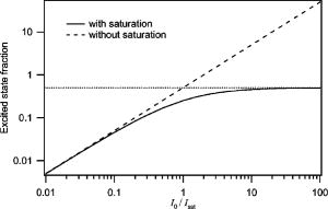

The key to understanding the saturation-induced changes in the size and profile of the observation volume, and thus the volume calibration in FCS, is to recognize that molecules at various locations within the focused laser excitation experience different photon fluxes, described by $S\left(\mathbf{r}\right)$ , and thus different degrees of saturation. Molecules at the center of the volume will experience a greater degree of saturation than those at the periphery of the focused excitation beam. Therefore, as saturation effects become significant, increases in the laser excitation power will effectively modify the distribution function describing the relative probability to detect fluorescence photons from various locations within the volume. Based on Eq. 1, the definition of the saturation intensity, and the assumption of the 3-DG observation volume for the unsaturated observation volume profile, the effective molecular excitation profile including the effects of saturation can be rewritten as:

Eq. 7

$${\widehat{W}}_{\mathrm{sat}}\left(\mathbf{r}\right)=(1+R_{\mathrm{sat}})\frac{{\widehat{W}}_{3\mathrm{DG}}\left(\mathbf{r}\right)}{1+R_{\mathrm{sat}}{\widehat{W}}_{3\mathrm{DG}}\left(\mathbf{r}\right)}.$$

Here we have defined a saturation parameter that specifies the degree of saturation in terms of the excitation and saturation intensities, with $R_{\mathrm{sat}}=I_0∕I_{\mathrm{sat}}$ . We note that we have made the simplifying assumption that the distribution functions in both the numerator and denominator of Eq. 7 can be represented by the same 3-DG distribution function. This is not physically precise, but as we show next, this approximation is very successful in fitting the experimental data. Given this success, together with the recognition that the 3-DG distribution itself is only an approximate description of the observation volume, this assumption is reasonable. We do anticipate that this approximation would break down at extremely high excitation rates. However, as a practical matter, the model works quite nicely over the full range of measured data shown next, and this range is already much wider than would typically be used in most FCS applications.

As shown in Figs. 3 and 4 , saturation can induce significant increases in the size of the observation volume as well as a flattening of the observation volume spatial profiles. The radial profile of this saturation-modified effective point-spread function can be seen in Fig. 3 for different excitation levels. For the lowest excitation intensity (below $I_{\mathrm{sat}}∕100$ ), the effective excitation profiles match the unsaturated profile precisely. At higher excitation, intensity changes in the size and shape of these profiles with increasing values of $R_{\mathrm{sat}}$ are dramatically apparent. Similar changes also occur in the axial profiles of the observation volume. Figure 4 shows surface plots of the volume distribution functions at two different saturation levels, highlighting the saturation-induced changes in both radial and axial volume profiles. At sufficiently high excitation intensities relative to the saturation intensity, the profiles acquire a flat top, and molecules within the flat region of the profile have reached the molecular brightness threshold.

Fig. 3

Saturation modified observation profiles show both increasing size and flatter profiles with increasing excitation intensity relative to the saturation intensity.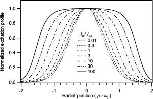

Fig. 4

Surface plots representing the size and shape of the observation volume: (a) the unsaturated 3-DG volume profile, and (b) the observation volume profile computed for excitation at ten times the saturation intensity.

The changes in the excitation profile will clearly alter the fluorescence observation volume, although the modified volume and gamma factors must be computed numerically, since there is not a simple analytical expression for the volume and gamma factors using the saturation-modified volume distribution function defined in Eq. 7. The absolute value of the volume depends explicitly on the beam waist of the focused laser excitation, although the scaling of the volume with $R_{\mathrm{sat}}$ does not. We therefore compute a volume scaling factor by dividing the computed volume by the corresponding nonsaturated volume. This scaling is plotted in Fig. 5 . For excitation intensity corresponding to 20% of the saturation intensity $(R_{\mathrm{sat}}=0.2)$ , the volume has already increased by 12% over its nonsaturated value. At the saturation intensity, the volume has increased by 50%, and at 10 times the saturation intensity, it is 350% (3.5 times) larger than the unsaturated volume. Saturation modifies not only the size of the measurement volume but the shape and hence the gamma factor as well. As the volume becomes larger, the boundaries become steeper with increasing values of $R_{\mathrm{sat}}$ resulting in a corresponding increase in the gamma factor. The scaling of the gamma factor with $R_{\mathrm{sat}}$ is plotted in Fig. 6 . Most important for FCS measurements is the ratio of the gamma factor divided by the volume. This quantity is also plotted in Fig. 6 and represents the expected amplitude scaling of measured fluorescence correlation curves for different values of $R_{\mathrm{sat}}$ .

Fig. 5

Scaling of the observation volume size with the degree of saturation.

Fig. 6

The gamma factor increases with increasing saturation due to the flattened volume profile. Also shown are the scaling factors for the beam waist and the ratio of the gamma factor divided by the volume. The bottom axis shows the degree of saturation, which represents the fundamentally important scaling. For reference, the top axis shows the average power on the sample computed for $532\text{-}\mathrm{nm}$ excitation with a $0.25\text{-}\mu \mathrm{m}$ beam waist and the saturation intensity computed for a dye with $5\times {10}^{-16}{\mathrm{cm}}^2$ cross section and $3.5\text{-}\mathrm{ns}$ excited state lifetime.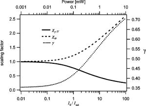

2.3.

Fluorescence Correlation Spectroscopy

Fluorescence fluctuation spectroscopy measurements are performed by monitoring the amplitude and time dependence of spontaneous equilibrium fluctuations in the fluorescence signal from the optically defined observation volume.^{1, 2} The fluctuation time scales of interest are typically much longer than the fluorescence lifetimes, and as such the fluctuation dynamics are determined mainly by local concentration fluctuations $\delta C(\mathbf{r},t)$ in molecular populations. The fluctuation signal is thus written:

Eq. 8

$$\delta F\left(t\right)=\psi \int {\widehat{W}}_{\mathrm{sat}}\left(\mathbf{r}\right)\delta C(\mathbf{r},t)d\mathbf{r}.$$

In FCS analysis, the information about the sample dynamics and kinetics is recovered through computation and analysis of correlation functions that are defined as:

Eq. 9

$$G\left(\tau \right)=\frac{⟨\delta F\left(t\right)\delta F(t+\tau )⟩}{{⟨F\left(t\right)⟩}^2}.$$

The general form of the normalized correlation function can normally be written as the product of two terms that represents the amplitude and the normalized relaxation time profile, i.e., $G\left(\tau \right)=G\left(0\right)A\left(\tau \right)$ . The amplitude factor can be expressed in the form $G\left(0\right)=\gamma ∕⟨C⟩V$ and is thus directly proportional to the ratio of the gamma factor divided by the volume and inversely proportional to the concentration. The temporal relaxation profile is governed by the physical and chemical relaxation processes in the sample, and also by the profile of the observation volume. For a purely diffusive system with a 3-DG observation volume, Eq. 9 has a simple analytical solution of the following form:

Eq. 10

$$G\left(\tau \right)=\frac{{\gamma }_{3\mathrm{DG}}}{⟨C⟩V_{3\mathrm{DG}}}\frac{1}{(1+4D\tau ∕{\omega }_0^2){(1+4D\tau ∕z_0^2)}^{1∕2}},$$

where $D$ is the molecular diffusion coefficient. This formula is widely used for curve fitting in FCS analysis.

There is no simple analytical form of the correlation function with the saturation-modified observation volume. However, correlation curves for arbitrary observation volume profiles can easily be computed numerically using the Fourier theory to evaluate the convolution integrals implicit in Eq. 9.¹³ We have performed these computations for the saturation-modified observation profiles and the results are shown in Fig. 7 . Saturation results in decreased correlation curve amplitudes due to the increased size of the observation volume. The temporal relaxation times are also increased due to the longer molecular crossing times associated with the larger volumes. The extended relaxation times can be more clearly seen in the inset, which shows the same correlation curves normalized to unit amplitude. Curves are shifted uniformly to the right with increasing degrees of saturation. We show next that these effects are indeed observed in one-photon FCS measurements, and that this modified theory can accurately account for the observed changes.

Fig. 7

Fluorescence correlation curves computed numerically based on the saturation modified observation volume profiles shown in Fig. 3. The correlation amplitudes decrease monotonically with increasing degree of saturation, represented by $R_{\mathrm{sat}}=I_0∕I_{\mathrm{sat}}$ . The inset shows the same curves normalized to unity to highlight the increasing relaxation time scales, with curves corresponding to larger values of the excitation intensity shifted to the right.

3.

Materials and Methods

Fluorescence correlation spectroscopy measurements were performed on our home-built inverted confocal microscope. The illumination source was a Millennia V $\mathrm{Nd}:\mathrm{Y}\mathrm{O}{\mathrm{V}}_4$ CW diode-pumped solid-state laser (Spectra-Physics, Mountain View, California). After $5\times$ beam expansion, the $532\text{-}\mathrm{nm}$ wavelength excitation light was focused in the sample with an objective lens (Olympus UApo $40\times$ water immersion, $\mathrm{NA}=1.15$ ), and the emitted light was collected by the same objective. The fluorescence signal was filtered, collected through a $10\text{-}\mu \mathrm{m}$ core diameter single-mode fiber, and sent to a fiber-coupled avalanche photodiode (SPCM-AQR-16-FC, EG&G, Vaudreuil, Canada). For the highest measurement powers, neutral density filters were also used in front of the fiber couplers to avoid saturating the detectors. The TTL outputs of the detectors were sent to an ALV correlator (Langen, Germany) to calculate correlation functions. The excitation power was adjusted by rotating a half wave plate in front of a linear polarizer. The power at the sample was calibrated and accounts for the known losses in various optical elements. Several autocorrelation curves were averaged at each excitation power and the standard deviations were estimated using published procedures.²⁰ Typical measurement times were a few minutes per autocorrelation trace. The sample used was rhodamine 6G dissolved in nanopure water $(18.2\mathrm{M}\Omega ∕\mathrm{cm})$ . The samples were filtered with $0.2\text{-}\mu \mathrm{m}$ filters before dilution to the final measured concentration, loaded into microbridge containers (Hampton Research, Aliso Viejo, California), and sealed with number 1.5 coverslips. The sample holder microbridges and coverslips were coated with blocker casein buffer (Pierce, Rockford, Illinois) to minimize the absorbance of dye molecules to the surfaces of the container. The concentration of the sample was determined using absorption measurements. All measurements shown in this work used the same mounted sample.

4.

Results and Discussion

To analyze the measured correlation curves and account for saturation, we need to find appropriate fitting functions based on the saturation-modified observation profiles introduced earlier. In principle, the correlation curves can be numerically computed within the curve fitting routine, although this results in prohibitively slow curve fitting procedures. Moreover, it is desirable to find simple curve fitting functions like Eq. 10 so they can be easily and widely adopted. We therefore introduce a curve fitting routine based on a simple modification of the widely used 3-DG correlation function [Eq. 10]. As shown in Fig. 7, excitation saturation modifies both the amplitude and the temporal relaxation of the correlation curves. Therefore, Eq. 10 is not adequate to simultaneously fit the full data series acquired at different $R_{\mathrm{sat}}$ values. However, we observe that Eq. 10 can in fact fit any one of the curves in Fig. 7 quite satisfactorily, even though this would result in unphysical variation in the recovered fitting parameters²¹ across the dataset. In other words, although saturation leads to excitation power-dependent calibration of the FCS instrumentation, we can reasonably fit the entire range of FCS curves with the 3-DG FCS model, provided we account for the excitation power-dependent scaling of the instrument calibration. We have already computed precisely how the correlation function amplitude scales with $R_{\mathrm{sat}}$ based on the saturation-modified volume profiles, and the results were plotted in Fig. 6. It is relatively straightforward to program this amplitude scaling into the fitting routines. We write this scaling factor as ${\chi }_{\gamma ∕V}$ , and the modified amplitude of the correlation function is thus given by the factor $G\left(0\right)=1∕⟨C⟩{\gamma }_{3\mathrm{DG}}∕V_{3\mathrm{DG}}{\chi }_{\gamma ∕V}$ . We note again that the value of the ${\chi }_{\gamma ∕V}$ scaling factor depends on the degree of saturation, which is dependent not only on the excitation intensity but also on the photophysical properties of the fluorescent molecule. Therefore, when saturation plays a role, the degree of saturation and thus the amplitude of measured correlation curves for molecules with different absorption cross sections or fluorescence lifetimes will be different even when excited using the same laser intensity.

We use a similar approach in finding scaling factors for the apparent beam waists under the influence of excitation saturation. The scaling of the beam waists accounts for the varied relaxation times of the correlation functions. To determine the appropriate scaling factors, the computed FCS curves in Fig. 7 were each fitted individually with the standard 3-DG correlation function from Eq. 10. The recovered values for the radial and axial beam waist, relative to the values used in computing the curves, provide the desired scaling rules. This operation results in finding the power-dependent scaling factors of the squared beam waists ${\chi }_{\omega }$ and ${\chi }_z$ with ${\chi }_{\omega }={\chi }_z$ . The values of the beam waist scaling factors are plotted in Fig. 6. The numerical values for each of the scaling factors are also reported in Table 1 . Below 1% of the saturation intensity, the values of the scaling factors are essentially one. At the saturation intensity, both the correlation amplitude (decreased) and the squared beam waist ( ${\omega }^2$ , increased) have changed by 22%, and at 10 times saturation intensity, the correlation amplitude has decreased by a factor of 2.3 and the squared beam waist has increased by 1.8 times relative to the unsaturated values. These scaling factors vary smoothly with $R_{\mathrm{sat}}$ , so intermediate values not found in the table can be determined by interpolation. For completeness, the table includes $R_{\mathrm{sat}}$ values up to 100, although we expect the model will break down before this very high degree of saturation. We report measurements up to an $R_{\mathrm{sat}}$ value of ten.

Table 1

Numerical values for the saturation-dependent scaling of the fluorescence correlation amplitudes χγ∕V and squared beam waists χω=χz with the degree of saturation Rsat .

Summarizing the new model, the saturation modified fitting function can be written as:

To analyze real experimental data, one must also account for triplet state transitions and/or photobleaching that can play an important role in FCS measurements, particularly at higher excitation rates. We therefore have implemented the widely used exponential correction factor for the triplet state kinetics in FCS.^{22, 23, 24} The effect of triplet state transitions on the correlation curves can be described by multiplying the diffusion-based correlation curve by the triplet correction factor: $(1-T+T{e}^{-\tau ∕{\tau }_T})∕(1-T)$ , where ${\tau }_T$ is the triplet correlation time and $T$ is the fraction of molecules occupying the triplet state. The triplet fraction and correlation times are not independent parameters, and they can be linked as $T=1-k{\tau }_T$ , where $k$ serves as a fitting parameter. This linking ensures that faster crossing into the triplet state corresponds to a higher triplet state fraction, and helps produce more stable fitting results. In the following data analysis, the full fitting function is therefore given by Eq. 11 multiplied by the triplet correction factor. Additional corrections for photobleaching were not required to fit the data.

We performed a series of FCS measurements for the rhodamine sample at different average laser powers. A subset of the measured curves and fits are shown in Fig. 8 . Many of the measured curves are omitted from this plot for visual clarity. We observed that the correlation amplitude was decreasing with increasing excitation power, as expected, demonstrating one of the effects of saturation. The temporal decay profiles of the measured correlation curves show the effects of both triplet crossing kinetics and saturation. The data in Fig. 8 were analyzed using a global fitting routine on the entire measured dataset using fitting functions as described before. The diffusion coefficient was held at its known value of $3\times {10}^{-6}{\mathrm{cm}}^2∕\mathrm{s}$ . The concentration and the beam waists of the unsaturated profile were global free parameters, as was the saturation intensity and the triplet linking parameter $k$ . The triplet correlation times were independent fitting parameters for each excitation power. The excitation intensity for each measurement was used as a fixed parameter in the fitting routines to calculate $R_{\mathrm{sat}}$ , as the saturation intensity parameter varied during fitting. The fits in Fig. 8 demonstrate that our FCS saturation model quite successfully characterizes the observed changes in the measured correlation functions, including the decreased correlation amplitudes and increased molecular crossing times associated with saturation. The same curves are plotted individually with residuals in Fig. 9 to show more clearly the fitting results. The recovered concentration was $65\mathrm{nM}$ and the beam waist was $0.17\mu \mathrm{m}$ . The recovered value for the saturation intensity corresponds to an average power of $60\mu \mathrm{W}$ . For a system with a $3.5\text{-}\mathrm{ns}$ fluorescence lifetime and $5\bullet {10}^{-16}{\mathrm{cm}}^2$ absorption cross section (typical values for a rhodamine dye), and $532\text{-}\mathrm{nm}$ excitation focused to this $0.17\mu \mathrm{m}$ beam waist, one would expect a saturation intensity that corresponds to an average power of $50\mu \mathrm{W}$ . This value thus compares favorably with the measured value. Figure 10 shows the recovered parameters for the triplet state crossing times and fractions. The trends in these parameters are physically reasonable. Given that we have only introduced a single additional free parameter compared with standard FCS analysis procedures that cannot account for saturation, the fitting results are remarkably accurate. We do observe small systematic deviations between the data and fits at the highest powers. This may be partly due to the limitations of the 3-DG model at the highest degrees of saturation, as well as limitations to the triplet crossing models. The triplet crossing theory assumes a constant fraction of molecules occupy the triplet state throughout the observation volume, which is clearly not the case. This may also at least partly explain the flattening of the recovered triplet crossing rate with increasing laser power at the highest excitation powers.

Fig. 8

A selection of the measured correlation curves for rhodamine 6G in water with widely varied excitation powers. They are plotted on a single graph to highlight the significant variation in amplitude and relaxation times for these measurements. The curves were fit with good success to the saturation-modified FCS theory.

Fig. 9

The correlation curves are the same data and fits shown in Fig. 8, plotted individually with residuals to show the fit quality.

Fig. 10

Recovered triplet state fraction and triplet crossing times for the data fits in Figs. 8 and 9.

The procedures introduced here suggest a slightly more sophisticated calibration procedure for FCS measurements. This involves measuring FCS curves at several different excitation powers. The beam waist and saturation intensity can then be determined through global fitting of this dataset. The recovered beam waist would be generally valid for all subsequent measurements with the same optics. On the other hand, the saturation intensity is dependent on the particular fluorescent molecules used and needs to be determined for each fluorophore either by measurement or via the known scaling of the saturation intensity with the absorption cross section and lifetime. Once the saturation intensity and the beam waist are known, both of which are independent of the diffusion coefficient, additional measurements can be easily analyzed individually using the saturation-modified fitting functions. One clear benefit of using the quantitative saturation model is that the parameters recovered through curve fitting are physically meaningful rather than simple fitting parameters. Its use can also help avoid systematic errors in data analysis if experimental requirements necessitate performing measurements at different excitation powers or with molecules of varied absorption cross sections.

It remains to be discussed how important these procedures will be in typical FCS experiments, and whether or not these findings can be more generally useful in FCS applications. One potential strategy for handling saturation in FCS measurements is simply to avoid its effects by working at excitation intensities well below the saturation intensity. We note that it is not always trivial to identify the limits of this “safe region” without a full analysis of the saturation intensity, since the competing effects of saturation and photobleaching or triplet kinetics sometimes make measured correlation curves appear to have constant amplitude, even when some saturation is occurring. Nonetheless, avoiding saturation once the saturation intensity is known can certainly be an effective strategy, provided that the measurement achieves a sufficient signal-to-noise ratio for such excitation rates. On the other hand, once the saturation intensity value is known, it is also straightforward to apply the theories introduced here. Moreover, higher signal-to-noise ratios are associated with higher excitation rates, and thus when the system under investigation is not harmed by higher power, this could be used advantageously while maintaining the capability to interpret measured results in terms of physically relevant parameters. Finally, this will have the added advantage that measurements need not be restricted to using fixed excitation powers to be interpreted accurately.

We believe that this capability to make measurements at multiple excitation levels and interpret them with quantitative accuracy can be extremely important in FCS applications. This is due to a general problem of model discrimination facing FCS analysis. When appropriate physical models are selected, very accurate information can generally be recovered through curve fitting of FCS data, but any particular measurement provides limited information that can be used to verify that correct fitting models are used. The capability to use the procedures introduced here to analyze FCS data with quantitative accuracy, even with changing excitation conditions, can provide an important tool for model discrimination in FCS analysis by testing whether recovered fitting parameters scale appropriately with excitation power. For example, if bleaching or triplet state models are included in a fitting analysis, one would expect that the bleaching or triplet crossing rates would increase proportionally with excitation power. Diffusion coefficients or chemical kinetic rates, on the other hand, should not change with excitation rates. It has not previously been possible to perform such tests, because changing the excitation power would change the instrument calibration in an unknown manner. We thus believe that use of the quantitative saturation theory results in important new capabilities for fluctuation spectroscopy analysis.

5.

Conclusions

We describe the effects of excitation saturation on one-photon FCS measurements in terms of the solutions to the photophysical rate equations, and introduce a simple curve fitting routine that allows FCS measurements to be analyzed while accounting quantitatively for the effects of excitation saturation. The fitting procedure is based on the commonly used 3-D Gaussian-based correlation functions with excitation power-dependent corrections to the FCS amplitude and relaxation times. We demonstrate that this approach is quite effective for analyzing FCS data acquired over a broad range of excitation conditions, while introducing only a single additional fitting parameter. As discussed earlier, the saturation-modified analysis also provides a useful new capability for model discrimination in FCS analysis.