1.

Introduction

Noninvasive mechanical property assessment is important to detect malignancy in tissue, for it is well known that tumors are characterized by an increase by many fold and anisotropy of the visco-elastic properties compared to normal tissue.^{1, 2} Imaging of elastic (and visco-elastic) properties to detect pathological changes in tissue is termed elastography. In elastographic imaging, the displacement or strain produced inside the object, owing to the application of an external force, is measured. The load applied is categorized under static or dynamic and can be applied either inside locally or on the boundary.^{3, 4, 5, 6, 7, 8} In static or quasistatic methods, either a constant load or a very low frequency vibratory force is employed. In dynamic methods, the forcing is either from a short duration pulse or harmonic vibration. Elastographic techniques are divided also on the basis of methods used to measure displacement or strain. On this basis, we have ultrasound (US) or sonoelastography,^{9, 10, 11} where an ultrasound imaging method is used to measure displacement, magnetic resonance elastography (MRE),^{12, 13, 14} which uses a phase-sensitive MR machine to measure displacement field and optical techniques such as speckle interferometry¹⁵ or optical coherence tomography (OCT),¹⁶ currently limited to measurements on surface or a few millimeters within. The efforts of different groups^{3, 4, 5, 17, 18, 19, 20} have resulted in the development of a noninvasive imaging modality that can distinguish malignant tumor from both normal tissue and benign tumor through mapping direction dependent elastic moduli of the tissue.

The principal advantage of an optical read-out mechanism compared to US- or MRI-based methods is its ability to measure displacements with a high degree of sensitivity, which is useful in resolving elastic property changes to a greater accuracy. The disadvantage is that light can hardly penetrate tissue, and an optical probe using OCT cannot measure displacement deep inside the tissue. A diffuse optical technique (DOT), which allows a much larger depth of interrogation, has not yet become popular as a measurement tool in optical elastography, because of light diffusion and consequent loss of image resolution. However, discrimination of photon paths through ultrasound tagging to determine whether they have intercepted a region of interest (ROI) or not has been made possible through the recently developed ultrasound-assisted optical tomography (UAOT).^{21, 22} This was used in optical property imaging with much larger spatial resolution. The method of UAOT can also be used to estimate the average displacement suffered by scattering centers in the volume insonified by a focusing US transducer, by measuring either the field or intensity correlation of the US tagged photons exiting the tissue. We have done simulations in our laboratory to compute field correlations and thus the intensity correlations of US-tagged photons, and received consistent results showing that the depth of modulation in the intensity correlation is related to the average amplitude of the vibrations of tissue constituents loaded by the ultrasound transducer in its focal region. This modulation depth can be used to estimate the average amplitude. Currently, we are doing experiments to establish the usefulness of US-tagged photons to measure displacements induced by a focusing US transducer employed for remote palpation deep inside the tissue. A brief outline of the described simulation is given in Sec. 2. We like to call elastography performed with US-tagged photons for displacement measurement as ultrasound assisted optical elastography (UAOE). The UAOE provides the background for the work presented here, which provides suitable tissue equivalent phantoms for preliminary trials of mechanical property mapping prior to moving to the clinic. In addition to UAOE, there are other application areas for the phantom presented in this work. One example is optical tomography assisted by US to provide a priori information on possible inhomogenities. Here, a trial phantom should have tailored optical and acoustic properties. Another possible application is in ultrasound elastography (or sonoelastography), which uses an ultrasound scanner to track displacements. Here, the phantom should match breast tissue for its mechanical and acoustic properties.

Phantoms are inanimate tissue-mimicking objects designed to match the tissue properties to be imaged, with variations to cover both normal and diseased states. DOT breast phantoms^{23, 24, 25} are designed to match optical absorption and reduced scattering coefficients of normal and cancerous breast tissue. The optical elastography phantoms for breast imaging applications should first of all match mechanical properties of breast in its normal and diseased states, and then, since the readout is diffuse light, it should also match the average optical properties of the tissue. Since ultrasound tagging is also employed, which fortuitously also helps to apply an approximation to a point load within the object, the phantom should be tailored to have proper acoustic properties matching the breast tissue. We report the development of an opto-elastic phantom that can be tailored to have stable mechanical properties to match both normal and cancerous regions of the breast, and almost independently, to have breast tissue-like optical and acoustic properties. Recently for photoacoustic imaging, a poly (vinyl alcohol)(PVA) gel phantom was developed, which was designed to have normal breast tissue scattering properties.²⁶ This was attained by subjecting a suitable mix of PVA concentrate and water through an appropriate number of freeze-thaw cycles. The freezing thawing cycles enhance cross-linking between polymer chains in the gel, which increases the mechanical strength of polymer.²⁷ In addition, owing to the large volume expansion because of freezing the water in the liquid phase of PVA in the cooling part of the freeze-thaw cycles, a number of pores are formed in the gel, increasing its turbidity. This is the genesis of a large scattering coefficient in the PVA gel so obtained.

The rest of the work is as follows. In Sec. 2, to substantiate the reason why such a phantom is important and useful for elastography with diffuse light probe for displacement measurement, we briefly describe the simulations performed by us to compute intensity correlations of light exiting a sample loaded by a focused US beam. In Sec. 3, we describe the method of preparation of the PVA gel, which is one of the standard methods from the literature,^{26, 27} pointing out also the steps in the recipe, which ensure proper elastic property variations. In Secs. 4, 5, we give the characterization of the optical and mechanical properties of the phantom. We discuss primarily the measurement and calibration of these properties and the variations we could achieve in the phantom. The properties discussed are the storage and loss moduli, refractive index, scattering coefficient, and the scattering anisotropy factor. Methods to measure the acoustic properties of the phantom such as average sound speed, attenuation coefficient for sound, and the acoustic impedance are given in Sec. 6. The measured properties are compared with reported data on normal and diseased breast tissue, wherever such data are available. Section 7 contains our concluding remarks.

2.

Simulation of Displacement and Elastic Property Estimation through Computing Ultrasound Tagged Photon Correlation

A tissue-mimicking phantom with homogeneous and isotropic background mechanical properties with two isotropic homogeneous inclusions of differing stiffness is insonified by a focusing ultrasound transducer. The phantom is assumed to have homogeneous optical absorption and reduced scattering coefficient throughout, equal to the average values of normal healthy breast tissue. The operating frequency of the transducer is fixed at $1\mathrm{MHz}$ . The ultrasound intensity in the focal volume of the transducer is estimated by solving the acoustic wave propagation problem through the medium, assuming average acoustic properties. This intensity is used to compute the ultrasound radiation force.^{5, 28} The forward elastography problem^{20, 29, 30} is solved for the region of insonification, assuming the Lame’s parameters in the region, under Dirichlet boundary conditions, which gives a distribution of displacement vectors in the insonified region. We found that the magnitude of the displacement is the maximum at the center of the focal volume, which dropped to very small values as we moved away from the center of the central lobe of the ultrasound focal spot. The direction of displacement, though it presented spatial variation, is predominantly toward the ultrasound propagation direction. The transducer is assumed to have a central hole, through which packets of photons are launched. Using Monte Carlo simulation, we have traced the photons through the phantom and collected the photons arriving at the detector (including the photons that passed through the focal region) on the boundary of the object in the direction of ultrasound. We have measured both the weight and overall pathlength of detected photons, from which the ensemble-averaged field correlation $⟨E(r,t)E(r,t+\tau )⟩$ , where averaging is done over the ensemble of photon paths, is computed using the recipe given by Wang.³¹ Intensity correlations $⟨I(r,t)I(r,t+\tau )⟩$ are then computed from field correlations. We have observed a distorted sinusoidal modulation on the correlation function when the ultrasound transducer was on. The strength of modulation, as observed in the Fourier transform of the correlation function at the US frequency, is found to be proportional to the average amplitude of the oscillations of the tissue constituents set in motion by the ultrasound, in the average direction of photon transport through the focal region. There are also other factors contributing to this modulation, such as refractive index and absorption coefficient modulations. In our simulations, where we have assumed the object to have no absorption coefficient variation, we have observed the following. When the elastic modulus in the focal region is increased, the computed displacement magnitude decreased proportionally. The intensity correlation function computed through Monte Carlo simulation showed a modulation whose strength is found to be proportional to the amplitude of displacement and nearly inversely related to the elastic modulus. Consistent results were obtained through repeated simulations, which showed clearly that strength of modulation in the intensity correlation could be used to readout the average displacement of particles, and through it to compute the mechanical properties such as elastic modulus or stiffness constant. We are currently doing experiments to substantiate these simulation results.

We would also like to make the following comments. 1. The amplitude readout is the average over the focal volume of the component in the average direction of photon transport. 2. As shown in the case of UAOT,³¹ the modulation depth in the intensity correlation is affected by local refractive index and optical absorption coefficient variation as well. However, for breast tissue, ${\mu }_a$ variation is small, ranging from ${\mu }_a=0.082\pm 0.007{\mathrm{mm}}^{-1}$ (for normal tissue) to ${\mu }_a=0.164\pm 0.017{\mathrm{mm}}^{-1}$ (for malignant tissue) at a wavelength of $\lambda =632.8\mathrm{nm}$ .³² But storage modulus variation is much larger, ranging from $20\pm 6\mathrm{kPa}$ (normal) to $301\pm 58\mathrm{kPa}$ (ductal carcinoma).¹ Therefore, for quantitative elasticity imaging, a way must be found to separate the contribution of displacement to the intensity modulation.

3.

Preparation of the PVA Phantom

The route taken to arrive at the polymerized stable form of vinyl alcohol, which itself does not exist in a stable form as a monomer, is given next. First, vinyl acetate is polymerized to poly (vinyl acetate) (PVAc), which hydrolyses to PVA. This last hydrolysis stage is seldom completed, so that the PVA stock specifies the degree of hydrolysis (usually above 98%), indicating that the stock is a mixture to that extent of PVA and PVAc. The degree of hydrolysis has an effect on the mechanical, chemical, and optical properties of the PVA gel obtained from the PVA stock.

PVA hydrogels are produced from PVA stock by enhancing the cross-linking between the polymer chains, which gives the PVA hydrogel greater mechanical strength. The gel so obtained, because of the network of cross-linked polymer chains, absorbs water and swells, but remains insoluble in water. Cross-linking can be promoted by such means as chemical agents (glutaraldehyde, acetaldehyde, and fomaldehyde), radiations from electron or gamma beams, or by physical cross-linking through providing conditions for crystallite formation. The chemical cross-linking leaves behind undesirable agent residues, and the mechanical strength achieved by irradiation is lower and nonuniform. Because of these reasons, we have used physical cross-linking of polymer chains through enhancing crystallite formation in PVA. Crystallite formation can be enhanced through subjecting the PVA aqueous solution to repeated freeze-thaw cycles. As the number and stability of crystallites are increased with the number of freeze-thaw cycles, the mechanical strength of the gel so formed (up to a point) is proportional to the number of cycles of freezing and thawing. In addition to the crystallite formation, the freeze-thaw cycles also promote repeated freezing of the coexisting water phase in the solution (with low PVA concentrate) and consequent expansion. This expansion leaves a number of pores behind, the distribution of which gives a turbid appearance to the PVA gel. Increasing the number of freeze-thaw cycles can also increase the turbidity up to an extent. We have prepared cross-linked and turbid PVA gels through employing repeated freeze-thaw cycles. Another parameter that can be profitably used to vary mechanical properties and possibly optical scattering property as well is the degree of hydrolysis of the PVA stock powder. We had two PVA powder stocks with 1. above 99% hydrolysis (from Sigma-Aldrich, USA, catalog number 363146, degree of hydrolysis $99+\%$ , average molecular weight 85,000 to 146,000) and 2. 98% hydrolysis (from Thomas Baker, Mumbai, India, article number 130086, degree of hydrolysis 98%, approximate molecular weight 125,000).

Aqueous solutions of PVA with concentration of 20% by weight were prepared in both cases by heating PVA and water over a temperature bath at $90\text{to}93°\mathrm{C}$ for $2\mathrm{h}$ with continuous stirring.^{26, 27} This solution was allowed to undergo repeated freeze-thaw cycles of freezing at $-20°\mathrm{C}$ for $12\mathrm{h}$ , followed by thawing at room temperature for $12\text{to}14\mathrm{h}$ . The number of cycles was increased from 2 to 7 to get the desired variations in mechanical, optical, and acoustic properties.

4.

Experimental Determination of Optical Properties

Generally, optical properties of the tissue or tissue-mimicking phantoms are determined by using so-called direct or indirect methods. The direct method is based on measurements of transmitted intensity variations and their analysis using simple analytical expressions for the same. Indirect methods make use of a theoretical model for light propagation in a medium, and attempt to solve simple inverse problems considering homogeneous material properties, with a view of obtaining a minimum error fit of the computed intensity variations to the measured intensity variations. We used a direct method for the determination of anisotropy factor $\left(g\right)$ and an indirect method based on the reverse Monte Carlo (MC) procedure for the determination of refractive index $\left(n\right)$ and scattering coefficient $\left({\mu }_s\right)$ . The angle-resolved transmission measurements can be used to determine the optical properties. To estimate ${\mu }_s$ , the measurement of $g$ is required. A reasonable estimate of $g$ can be arrived at by fitting the experimentally obtained scattering phase function to the Heney-Greenstien (H-G) phase function (the most widely used parametric phase function). The H-G function is valid in the limit of single scattering. For indirect measurements, a model of light transport is required to deduce the optical parameters for which Monte Carlo simulation is used. The measurement of transmitted intensity for various theta values are made on optically thick samples. Using the value of $g$ already obtained, ${\mu }_s$ and $n$ are determined by comparing the experimental data with the results of Monte Carlo simulations.

4.1.

Experimental Setup

The experimental setup for measuring both ${\mu }_s$ and $g$ has provision for illuminating the sample from a He–Ne laser $(\lambda =632.8\mathrm{nm})$ . Light is modulated at a frequency of $800\mathrm{Hz}$ by a chopper included in front of the laser to facilitate lock-in detection of the output. The detector is mounted on a theta stage with the capability of angle-resolved measurement up to $0.5\mathrm{deg}$ . In front of the detector, there is a light gathering system with a collection lens. The overall acceptance angle of the detector system used is $2.8\mathrm{deg}$ . The schematic diagram is given in Fig. 1 .

Fig. 1

The experimental setup for determining the optical properties. The He–Ne laser transilluminates the sample, which is mounted on a theta stage. The detector with the collecting lens is used to measure the angle-resolved intensity. The chopper is used to facilitate lock-in detection of intensity. The same setup is used to measure $I\left(\theta \right)$ from both thick and thin samples.

For angle-resolved intensity measurements, we use samples of PVA gels made from PVA concentrates of both 99% hydrolysis and 98% hydrolysis and different freeze-thaw cycles. Each sample is mounted on a sample holder so that the light is incident perpendicular ( $0\text{-}\mathrm{deg}$ angle of incidence). With the detector on the theta stage, we measure intensity with respect to theta, for theta going from 0 (normal exitance) to $90\mathrm{deg}$ . Each measurement is the average of half a dozen readings.

In the case of ${\mu }_s$ and $n$ measurements, relatively thicker samples are used. Two different samples of thickness 1.2 and $2.2\mathrm{cm}$ are used for each category of the phantom, and the transmitted intensity is measured and again averaged to get $I_E\left(\theta \right)$ . Angle-resolved intensity measurements from samples of the gel with increasing number of freezing thawing cycles, i.e., with increasing turbidity, are taken.

4.2.

Results of Optical Property Measurements

The value of $g$ is extracted using the Henyey-Greenstein (H-G) phase function, where the exit angle dependence of transmitted intensity is expressed as (in the limit of single scattering)

$$I\left(\theta \right)=K\left[\frac{1-g^2}{{(1+g^2-2g\cos \theta )}^{3∕2}}\right].$$

To satisfy the condition of single scattering, the samples are cut to thicknesses of approximately $150\mu \mathrm{m}$ (for stiffer samples) and $500\mu \mathrm{m}$ (less rigid samples). Of all the sets of phantoms fabricated, some of the samples prepared from 98% hydrolysis stock were not rigid enough to be properly cut to very thin samples. All the stiffer samples are cut to thickness $\sim 150\mu \mathrm{m}$ , and the softer ones to $\sim 500\mu \mathrm{m}$ . The variation of the mean scattering length (estimated later through ${\mu }_s$ ) in the softer material is observed to be between 700 and $400\mu \mathrm{m}$ . In the stiffer samples, the estimated mean scattering length varied between 400 and $160\mu \mathrm{m}$ . For the stiffer samples, the single scattering assumption is fully justified; it is not so in the few softer ones. The experimentally obtained $I_E\left(\theta \right)$ is fitted to the theoretical H-G function to get the value of $g$ using a constrained optimization search (the MATLAB function “fmincon” is used) to minimize $\Delta I={\parallel I_E-I\parallel }^2$ , with proper initial guess and lower and upper bounds for both $K$ and $g$ . Figure 2 shows a typical, experimentally obtained transmitted intensity and its fit using the H-G phase function. The value of $g$ obtained for the 98% hydrolysis phantom is 0.89, and that for 99% hydrolysis phantom is in the range of 0.9 to 0.9259 for different freeze-thaw cycles.

Fig. 2

Angle-resolved normalized intensity transmittance measured from a thin sample. The open circles represent the experimental data and the solid line gives the final fit for the experimental curve using the Henyey Greenstein scattering phase function. The sample is prepared from 99% PVA stock, subjecting it to five freeze-thaw cycles.

In addition to $I_E\left(\theta \right)$ , the experimentally obtained angular intensity distribution from thick phantom samples, theoretical distributions of intensity $I_c\left(\theta \right)$ are also computed using MC simulation of photon transport through similar phantoms. The background optical properties such as, ${\mu }_s$ , ${\mu }_a$ , and $n$ used in the simulations are, ${\mu }_a=0.08{\mathrm{mm}}^{-1}$ , ${\mu }_s=13{\mathrm{mm}}^{-1}$ , and $n=1.35$ , which correspond to reported averaged properties for healthy breast tissue.^{32, 33, 34} The optical properties ${\mu }_s$ , ${\mu }_a$ , and $n$ are adjusted to fit $I_c\left(\theta \right)$ to $I_E\left(\theta \right)$ by a Levenberg-Marquardt procedure, which minimized $\Delta I={\parallel I_E-I_C\parallel }^2$ . The ${\mu }_s$ , ${\mu }_a$ , and $n$ values, which gave the minimum $\Delta I$ , are retained as the measured optical properties. Figure 3 shows a typical $I_E\left(\theta \right)$ curve along with the fit obtained through MC simulation. The ${\mu }_a$ value obtained is of the order of $0.004{\mathrm{mm}}^{-1}$ $(\lambda =632.8\mathrm{mm})$ , much less compared to the reported average value for normal breast tissue.^{32, 34} One can increase ${\mu }_a$ by adding a suitable dye such as Ecoline,³⁵ as in the case of optical tomography phantoms or phantoms for photoacoustic imaging. For a better mimic of breast tissue, ${\mu }_a$ also should be tailored. We have not done this in our present study, and concentrated only on matching scattering coefficient, refractive index, and elastic properties. The extracted ${\mu }_s$ and $n$ values for the different samples fabricated are given in Tables 1 and 2 .

Fig. 3

The normalized angle-resolved intensity transmittance from a thick sample. Open circles represent the experimental data and the solid line gives the final fit for the experimental data, arrived at by calculating $I\left(\theta \right)$ using Monte-Carlo simulation. The sample is prepared from 99% PVA stock, subjecting it to five freeze-thaw cycles. The extracted optical properties are $g=0.9259$ , $n=1.36$ , and ${\mu }_s=6{\mathrm{mm}}^{-1}$ .

Table 1

Optical properties of the phantoms fabricated using 99+% hydrolysis PVA stock for different freeze-thaw cycles (wavelength=632.8nm) . For comparison, for normal breast tissue μs′ in mm−1 is 0.87±0.22 at 750nm (in vivo),38 and 1.57±0.13 at 630nm (in vitro),32 g is 0.88 at 632.8nm (in vitro),32 and n=1.33−1.55 at 589nm .33 The values for malignant breast tissue are μs′ in mm−1 is 2.62±0.15 and g=0.96 at 630nm (in vitro).32

Numberoffreeze-thawcycles	Scatteringcoefficient (μsmm−1)	Anisotropyfactor (g) σ=±0.0050	Reducedscatteringcoefficient (μs′mm−1)	Refractiveindex (n) σ=±0.001
2	$2.53\pm 0.013$	0.9000	$0.253\pm 0.014$	1.36
3	$3.66\pm 0.101$	0.9000	$0.366\pm 0.029$	1.36
4	$4.89\pm 0.111$	0.9000	$0.488\pm 0.036$	1.36
5	$5.08\pm 0.131$	0.9100	$0.457\pm 0.038$	1.36
6	$6.00\pm 0.087$	0.9259	$0.445\pm 0.037$	1.36

Table 2

Optical properties of the phantoms fabricated using 98% hydrolysis PVA stock for different freeze-thaw cycles (wavelength=632.8nm) . For comparison with normal and malignant breast tissue properties, see the note at the end of the caption for Table 1.

No. offreeze-thawcycles	Scatteringcoefficient (μsmm−1)	Anisotropyfactor (g) σ=±0.0030	Reducedscatteringcoefficient (μs′mm−1)	Refractiveindex (n) σ=±0.002
2	$1.441\pm 0.120$	0.8900	$0.159\pm 0.018$	1.34
3	$2.457\pm 0.054$	0.8900	$0.280\pm 0.023$	1.34
4	$2.533\pm 0.012$	0.8900	$0.279\pm 0.009$	1.34
5	$2.778\pm 0.115$	0.8900	$0.306\pm 0.005$	1.34
6	$3.670\pm 0.079$	0.8900	$0.404\pm 0.020$	1.34
7	$4.500\pm 0.076$	0.8900	$0.495\pm 0.022$	1.34

5.

Experimental Determination of Mechanical Properties

Soft tissues are characterized as incompressible, visco-elastic materials likely to undergo large deformations.³⁶ Assuming the material shows linear visco-elastic behavior, the response of the material (either displacement or strain) to a sinusoidally varying stress superimposed on a constant load will also be sinusoidal. In other words, if the applied stress varies as $\sigma \left(t\right)=a+{\sigma }_0\sin \omega t$ , the resultant strain response will be $\epsilon \left(t\right)={\epsilon }_0\sin (\omega t+\delta )$ , where ${\sigma }_0$ and ${\epsilon }_0$ are the maxima for applied stress and observed strain, respectively. The observed phase shift $\delta$ in $\epsilon \left(t\right)$ compared to $\sigma \left(t\right)$ is a reflection on the viscous behavior of the material. For the purely elastic case, $\delta =0$ , which implies that the applied stress is directly proportional to and in phase with the observed strain.

5.2.

Results of Mechanical Property Measurements

The experimentally measured storage moduli $\left(E^{\prime }\right)$ are given in Tables 3, 4 for $99+\%$ hydrolysis and 98% hydrolysis, respectively. When we used 98% hydrolysis PVA as the starting material with freeze-thaw cycles increasing from 2 to 7, the $E^{\prime }$ increased from $11.39\text{to}97.28\mathrm{kPa}$ (Table 4). In the case of $99+\%$ hydrolysis PVA with freezing-thawing cycles varying from 2 to 6, the variations in $E^{\prime }$ are from $65\text{to}162\mathrm{kPa}$ (Table 3). The measured values of loss modulus $\left(E^{″}\right)$ for the previous cases are also given in Tables 3, 4. Figure 4 shows, for a typical sample, the measured variation in the storage and loss moduli with time.

Fig. 4

The measured variations in storage $\left(E^{\prime }\right)$ and loss $\left(E^{″}\right)$ moduli with respect to time (the result of a time-sweep measurement). The sample is PVA gel of cylindrical shape with diameter $6\mathrm{mm}$ and height $15\mathrm{mm}$ , prepared from $99+\%$ PVA stock, subjecting it to three freeze-thaw cycles. Sinusoidal loading is kept at a frequency of $3\mathrm{Hz}$ . (There is almost no variation noticeable in either $E^{\prime }$ or $E^{″}$ with time.) The value of $E^{″}$ is much smaller than $E^{\prime }$ , which is similar to the behavior of actual breast tissue.¹

Table 3

Visco-elastic properties of the phantoms fabricated using 99+% hydrolysis PVA stock for different freeze-thaw cycles (frequency 3Hz ). Elastic moduli (kPa) of normal and malignant breast tissue1 (measured with 20% precompression and frequency of 1Hz ) are for: 1. normal fat 20±6 ; 2. normal glandular tissue 57±19 ; 3. fibrous tissue 232±16 ; 4. ductal carcinoma 301±58 .

Number offreeze-thawcycles	StoragemoduluskPa	LossmoduluskPa	tanδ
2	$65.49\pm 1.09$	$5.40\pm 0.25$	$0.0827\pm 0.0031$
3	$135.19\pm 2.78$	$7.00\pm 0.20$	$0.0515\pm 0.0014$
4	$162.67\pm 1.02$	$8.85\pm 0.23$	$0.0539\pm 0.0015$
5	$149.99\pm 2.12$	$5.77\pm 0.13$	$0.0384\pm 0.0009$
6	$149.00\pm 0.97$	$12.90\pm 0.18$	$0.0867\pm 0.0006$

Table 4

Visco-elastic properties of the phantoms fabricated using 98% hydrolysis PVA stock for different freeze-thaw cycles (frequency 3Hz ). For comparison with normal and malignant breast tissue properties, see the note at the end of the caption for Table 3.

No. offreeze-thawcycles	StoragemoduluskPa	LossmoduluskPa	tanδ
2	$11.39\pm 0.81$	$2.52\pm 0.16$	$0.2213\pm 0.0094$
3	$23.42\pm 0.82$	$4.35\pm 0.20$	$0.1857\pm 0.0027$
4	$40.35\pm 1.34$	$6.10\pm 0.54$	$0.1511\pm 0.0067$
5	$43.73\pm 0.41$	$8.24\pm 0.11$	$0.1884\pm 0.0043$
6	$51.18\pm 0.82$	$5.91\pm 0.39$	$0.1154\pm 0.0040$
7	$97.28\pm 1.23$	$16.37\pm 0.40$	$0.1683\pm 0.0058$

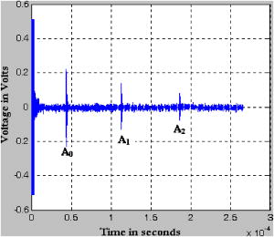
We do not have data on $E^{″}$ (loss modulus) of breast tissue, except that $E^{″}$ is very small^{1, 36} for normal breast tissue compared to $E^{\prime }$ . (This is found to be true for all the samples that we have prepared.) Therefore, a comparison to changes in $E^{″}$ in breast due to pathology is presently not possible. But for $E^{\prime }$ , the storage modulus, the available literature tells us that the variations in breast tissue are from $11\text{to}25\mathrm{kPa}$ (for normal fat), $14\text{to}42\mathrm{kPa}$ (for fibrous tissue), and $74\text{to}138\mathrm{kPa}$ (for invasive and infiltrating ductal carcinoma).³ This clearly shows that a PVA gel phantom can be tailored to have $E^{\prime }$ matching either normal breast tissue or malignant ones. This match is an important requirement when we are looking for materials for tissue-mimicking phantoms for elastography.

6.

Experimental Determination of Acoustic Properties

The specific acoustic properties commonly used to characterize a tissue mimicking material are the velocity of ultrasound in the medium, sound attenuation coefficient, and the acoustic impedance. In medical acoustics, the attenuation coefficient is expressed in dB/cm/MHz. Acoustic impedance is important in the determination of acoustic transmission and reflection at the boundary between an object and the surrounding medium, or between different materials that make up a composite object.

6.1.

Measurement Methods

The measurement scheme uses a series of single element focusing transducers for different frequencies and a pulser-receiver set capable of generating and detecting pressure waves at the desired frequencies (HF-400 high frequency pulser-receiver, Roop Telsonic Ultrasonix Limited, Mumbai, India). The experimental setup is schematically shown in Fig. 5 .

Fig. 5

The schematic of the experimental setup used to measure acoustic properties of the phantom. The sample is immersed in water to provide impedance matching. The ultrasound pulser provides $2.2\text{-}\mathrm{MHz}$ pulses with pulse repetition frequency of $1\mathrm{kHz}$ . The reflected pulses from the sample-water interfaces (front and back surfaces of the sample) are also detected by the transmitter/receiver combination.

The sound velocity is measured using the pulse-echo technique. The phantom, as well as the transducer, is immersed in a tank of distilled water, where water is used as the coupling medium between the phantom and the transducer. The received pulses are displayed on an oscilloscope (Tektronics TDS 3032B). The ultrasound transducer, which functions as both transmitter and receiver, generates the ultrasound pulses, which make multiple roundtrips through the sample, producing echoes. The velocity of sound in the phantom is derived from the observed roundtrip transit time $\delta t$ , and the measured thickness of the specimen $L$ , as $c_s=2L∕\delta t$ .

This setup can also be used to measure the sound attenuation coefficient and the acoustic impedance of the PVA gel. For this, we measure the amplitude attenuation suffered by the echoes from the gel when insonified by an ultrasound pulse. The origin and composition of the echoes can be understood by noting that the first two echo pulses are those reflected from the front and back surfaces of the phantom, and subsequent pulses are from the trapped pulse within the phantom reflected from the back and transmitted through the front surface of the phantom. Assuming that $A_0$ , $A_1$ , and $A_2$ are the amplitudes of the first three echoes, respectively, (as shown in Fig. 6 ), the attenuation coefficient of the gel in decibels per centimeter (at frequency of insonification) is given by³⁷

$$\alpha =\frac{\ln (R∕B2)}{2L},$$

where $R$ is the reflection coefficient of water-phantom interface, given by

$$R={\left[\frac{B_0{B}_2}{1+B_0{B}_2}\right]}^{1∕2},\text{where}{B}_0=\frac{A_0}{A_1},B_2=\frac{A_2}{A_1}.$$

Since the reflection coefficient of the phantom with respect to water is $R=Z_2-Z_1∕Z_2+Z_1$ , where $Z_1$ and $Z_2$ are the acoustic impedance of water and phantom, respectively, the measured $R$ helps us arrive at the acoustic impedance of the phantom from the known acoustic impedance of water. We have cross-checked the previous impedance measurement by measuring the density $\left(\rho \right)$ of the phantom with the Mettler Toleto density kit and calculating the impedance of the phantom as $Z_2=\rho c_s$ , where $c_s$ is the measured velocity of sound in the phantom.

Fig. 6

Typical reflected pulses received by the pulser receiver. The transit time $\delta t$ is measured from the oscilloscope.

7.

Discussions and Conclusion

We fabricate and test PVA gel phantoms whose mechanical, optical, and acoustic properties can be tailored to match those of human breast tissue by adjusting the number of freeze-thaw cycles and the degree of hydrolysis of the starting PVA stock. We are able to vary the mechanical and optical properties of the phantom to match those of healthy and malignant breast tissue. Such a phantom is very useful for preclinical experiments to prove some of the methods that use more than one imaging modality, such as optical tomography, with region of interest a priori determined using an ultrasound imager, sonoelastography, photoacoustic imaging, or optical elastography as planned in our laboratory. The phantom is also tailored to mimic average acoustic properties of healthy breast tissue. Malignancy does not produce a large variation in sound speed in tissue, and therefore a match of sound speed of normal average healthy breast tissue is considered adequate for the phantom. This is not the case with acoustic impedance, which varies not only from normal tissue to diseased one but also from one type of healthy tissue to another. Therefore for acoustic impedance, the phantom does not truly represent the heterogeneous breast tissue but has only an average homogeneous property.

The mechanism responsible for varying the mechanical strength of the material, which is physical cross-linking of the PVA chain, can be controlled by either varying the number of freeze-thaw cycles or the degree of hydrolysis in the PVA stock. But both these parameters also affect the density of pore formation, which gives the phantom its scattering property. Our observation is that the mechanical strength is very strongly dependent on the degree of hydrolysis, and turbidity similarly on the number of freeze-thaw cycles. We had only two PVA stock powders, one with above 99% hydrolysis and the other with 98%. With these and by varying the number of freeze-thaw cycles from two to six, we could get samples with the same ${\mu }_s$ values and different storage modulus values as given in Table 7 . If the degree of hydrolysis can be further varied, it should also be possible to get samples of same storage modulus with varying scattering coefficient values.

Table 7

Sample pairs showing same or similar scattering coefficient values but differing in mechanical strength obtained through varying freeze-thaw cycles and degree of hydrolysis.

Phantoms can also be produced with included stiffness inhomogeneities (at the moment it is not possible to maintain the scattering property in the inclusion to that of homogeneous background material). For example, if we want a stiffer inclusion with $E^{\prime }=97\mathrm{kPa}$ for the tumor and a homogenous background at $11\mathrm{Kpa}$ for normal tissue, the recipe is as follows. With 98% hydrolysis stock, prepare a cylinder for the tumor with five freeze-thaw cycles. Place this cylinder in the mold in the appropriate location where it is required, fill the gap with the stock solution, and continue the freeze-thaw cycles twice more. As seen from Table 4, the background material, which had only two freeze-thaw cycles, will have $E^{\prime }=11\mathrm{kPa}$ and the inclusion, which received seven freeze-thaw cycles, will have $E^{\prime }=97\mathrm{kPa}$ .

In conclusion, a better understanding of mechanical cross-linking and pore formation, and their control through varying freeze-thaw cycles and degree of hydrolysis is needed to be able to fine-tune mechanical and optical properties of the phantom and possibly control them independently.