Fluorescence resonance energy transfer imaging via fluorescence polarization measurement

Meir Cohen-Kashi; Yaniv Namer; Mordechai Deutsch

doi:10.1117/1.2209955

1 May 2006 Fluorescence resonance energy transfer imaging via fluorescence polarization measurement

Meir Cohen-Kashi, Yaniv Namer, Mordechai Deutsch

Author Affiliations +

Journal of Biomedical Optics, Vol. 11, Issue 3, 034015 (May 2006). https://doi.org/10.1117/1.2209955

Abstract

Fluorescence resonance energy transfer (FRET) has become a widely used spectroscopic tool for detecting molecular interactions and molecular proximity in solution, as well as in membranes. On the other hand, fluorescence polarization (FP) is a convenient measure: ratiometric and simple to execute. This work presents a novel methodology for determining energy transfer efficiency (E) via FP measurement. The methodology is based on the fact that a donor's fluorescence lifetime is shortened due to FRET and, consequently, its FP increases. As a model, the present work evaluates the E between fluorescein and rhodamine conjugated ConA attached to the receptors in the lymphocyte membrane. It shows not only that FRET imaging via FP is possible, but also that it is inexpensive, simple to perform, conveniently adaptable to the commonly used fluorescent microscopy, and readily interpretable.

1. Introduction

Fluorescence resonance energy transfer (FRET) is widely used as a spectroscopic tool for detecting molecular interactions and molecular proximity in solution, as well as in membranes. It involves the nonradiative transfer of energy from an excited donor molecule to an appropriate acceptor.¹ Microscopic FRET imaging methods currently used to measure energy transfer are based on monitoring donor photobleaching,² variations of sensitized acceptor fluorescence,³ donor quenching,⁴ donor lifetime,⁵ and fluorescence polarization (FP).⁶ In principle, the measurement of FRET using a microscope is as informative as the current macroscopic FRET measurements; however, it enables the visualization of the spatial distribution of FRET efficiency over the entire image, rather than averaging the values over the whole object and/or object population. Since energy transfer is possible in the distance range of 1 to $10 nm$ between the donor and acceptor, an additional increase in spatial resolution is enabled. This is a unique advantage of FRET imaging, allowing to resolve distances and interactions down to a molecular level.⁷

In the present study, FRET was imaged using a method developed for a wide-field microscope, which we modified for FP measurement. In an earlier study, we proposed a methodology for a direct determination of the efficiency of energy transfer (E) via FP, and showed its correlation with other techniques.⁶

Briefly, FP is defined as the ratio:

Eq. 1

(I_{‖} - I_{⊥}) ∕ (I_{‖} + I_{⊥}),

where

(I_{‖})

and

(I_{⊥})

are, respectively, the emitted fluorescence intensities

(I)

parallel and perpendicular to the excitation field vector. Practically, FP measures the level of anisotropy of fluorophores hosted in a medium. Hence, the less the fluorophore rotates relative to the excitation field during its fluorescence lifetime (FLT), the higher its FP. Eventually, the more restricted the rotational movement and/or the shorter the FLT, the higher the FP value, and vice versa.

Fluorescence energy transfer in itself provides an additional pathway for the evacuation of the fluorescent donor’s excited state, thus shortening the donor’s FLT, and consequently raising its emitted FP. We used this increase in the FP of the donor to show that E can be evaluated by the following formula⁶:

Eq. 2

E = \frac{P_{0} (P_{D}^{A} - P_{D})}{P_{D}^{A} (P_{0} - P_{D})},

where

P_{0}

is the FP limit value of the donor in a frozen gas-like system, and

P_{D}

and

P_{D}^{A}

are the FP of the donor in the absence and presence of the acceptor, respectively. (Appendix A provides a complete derivation of this equation.) Others utilized the acceptor’s FP to qualitatively rather than quantitatively follow alterations in E values.⁸

The advantages of such a technique are that the FP measurement is ratiometric, simple, predictive, and insensitive to inner-filter effects,⁹ and the determining of E through it is inexpensive, simple to perform, conveniently adaptable to the commonly used fluorescent microscopy, and readily interpretable,⁶ as is presented in this study.

2. Material and Methods

2.1.

Cells

The Human Molt 4 T-lymphoblast cell line was grown in a humidified atmosphere containing 5% ${CO}_{2}$ , in RPMI 1640 medium (Biological Industries, Israel); supplemented with 10% (v/v) heat-inactivated fetal calf serum (Biological Industries, Israel), 2-mM L-glutamine, 50-U/ml penicillin, and $100 μ g ∕ ml$ streptomycin. The cells were washed by centrifugation for $5 \min$ at room temperature through $5 ml$ of phosphate buffered saline (PBS), the supernatant was removed, and cells were resuspended in cold PBS at a concentration of $6 . 10^{6} ∕ ml$ and kept at $4 ° C$ until labeling with concanavalin A.

2.2.

Concanavalin A

Nonconjugated concanavalin A (ConA), fluorescein conjugated ConA (ConA-F), and tetramethylrhodamine conjugated ConA (ConA-R) were purchased from Vector (Burlingame, California).

2.3.

Cell Labeling

Two kinds of samples were prepared: 1. cells labeled with a mixture of the same amounts of ConA-F and ConA-R (double-labeled cells); and 2. cells labeled with a mixture of the same amounts of ConA-F and nonfluorescent ConA (F-single labeled cells), or else, ConA-R and nonfluorescent ConA (R-single-labeled cells). The nonfluorescent ConA was added to preserve the same total ConA concentration. The labeling of the samples was performed at $4 ° C$ during $30 \min$ . The total concentration of ConA was $200 μ g ∕ ml$ in each type of experiment.

After labeling, cells were washed free of ConA by centrifugation for $5 \min$ at $4 ° C$ through $5 ml$ of PBS. The supernatant was removed and cells were resuspended in cold PBS. Finally, samples were fixed in 4% formaldehyde at room temperature, washed again under the prior conditions, and resuspended in 80- $μ l$ cold PBS supplemented with vitamin C at a final concentration of $10 μ M$ to prevent photobleaching. The labeled cells were maintained at $4 ° C$ until their loading onto a slide for microscopic measurement.

2.4.

Imaging Instrumentation

Cells were imaged using an epifluorescence microscope (BX61, Olympus, Japan), with a $20 \times 0.4$ -NA LCPlanFl objective (Olympus, Japan) and 100-W xenon lamp (Olympus, Japan). Images were collected by the photometric ${CoolSNAP}_{H Q}$ monochrome charge-coupled device (CCD) camera with a $1392 \times 1040$ imaging array and $6.45 \times 6.45$ - $μ m$ pixels (Roper Scientific, Incorporated, Trenton, New Jersey). This cooled CCD camera system provides 12-bit digitalization at two pixel rates: 10 and $20 MHz$ .

ConA-F and ConA-R were detected using an appropriate filter set, namely F filter cube (excitation 470 to $490 nm$ , 505-nm long-pass dichroic, emission 510 to $530 nm$ ) and R filter cube (excitation 510 to $560 nm$ , 565-nm long-pass dichroic, emission 577 to $632 nm$ ), respectively. The filters were purchased from Chroma Technology Corporation (Brattleboro, Vermont). The control of the microscope, filter and polarizer wheels, data acquisition and processing, including FP calculations, were performed using in-house macros written for the Image-Pro Plus (IPP) software (Media Cybernetics, Incorporated, Silver Springs, Maryland).

For FP measurements, the microscope was modified as follows: a polarizer (Edmond Industrial Optics, Barrington, New Jersey) was inserted across the excitation beam, and two polarizers (analyzers) were installed in a motorized computer-controlled filter wheel (Olympus, Japan), and inserted across the emitted fluorescence beam (see Fig. 1 ). These two emission polarizers were oriented parallel and perpendicular to the direction of the excitation polarization. The exchange of the analyzers was done by the filter wheel, positioning the polarizers across fluorescence emission at a correct time.

Fig. 1

The measurement system. Excitation light from the Xe lamp passes through a polarizer (Ex. Pol.) and an excitation filter (ExF) and impinges on a dichroic mirror (DM). Light reflected by the DM passes through an objective and illuminates the cell sample positioned on the slide. The partially polarized fluorescent light emitted from the cells is collected by the objective, and passes through the DM, emission filter (EmF), and then through a polarization analyzer (PA) to the CCD.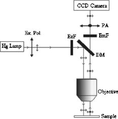

2.5.

Data Acquisition

In the following, $F I_{‖}$ denotes images acquired when the excitation and emission polarizers are parallel, whereas $F I_{⊥}$ denotes images obtained when they are perpendicular to each other.

Four images must be obtained during a FRET experiment: $F I_{‖}$ and $F I_{⊥}$ images from single-labeled cells, denoted by $F I_{‖}^{F}$ and $F I_{⊥}^{F}$ , respectively; and $F I_{‖}$ and $F I_{⊥}$ images from double-labeled cells, denoted by $F I_{‖}^{F R}$ and $F I_{⊥}^{F R}$ , respectively.

2.6.

Data Analysis

To obtain E mapping cell images, we must first derive FP images from the FI images mentioned before. Eventually, from the FP images, the values of E are calculated according to Eq. 2, pixel by pixel, as described next.

2.7.

Fluorescence Polarization Imaging

FP images were obtained using the imaging mathematics, from the $F I_{‖}^{F}$ , $F I_{⊥}^{F}$ , $F I_{‖}^{F R}$ , and $F I_{⊥}^{F R}$ images. First, the images were converted from 12-bit grayscale to a floating point format, from which a constant corresponding to background (e.g., scattered light and camera dark current) was subtracted. The background was evaluated by averaging over a nonstained sample image, taken under the same experimental conditions, and was found to be $134 au$ .

Then, a computerized segmentation procedure was applied on the $F I_{‖}$ image, selecting bright patches on the cell membrane, and creating a filtered $F I_{‖}$ image, which shows only the bright patch areas. To create a spatial binary mask, a value of unity was attributed to the selected bright patches on the filtered $F I_{‖}$ image, while null values were attributed to remaining cellular areas. For further analysis, the latter defined mask is multiplied by the $F I_{⊥}$ image to generate a filtered $F I_{⊥}$ image.

Eventually, a calculated filtered FP $(F P_{f})$ image is obtained by processing the filtered $F I_{‖}$ and $F I_{⊥}$ images via the following formula:

Eq. 3

F P_{f} = \frac{F I_{‖} - M F I_{⊥}}{F I_{‖} + M F I_{⊥}} .

Here,

M

is the microscope correction factor that compensates for the distortion of FP measurement due to the microscope optical arrangement and numerical aperture (NA).^{6, 10} Practically, to calculate the

M

value, the intensity of unpolarized light (the transmitted microscope illumination light) was recorded by the camera at two perpendicular directions of polarization, as two images

I

and

I_{⊥}

. Then, the

I

image was divided by

I_{⊥}

to give the

M = I ∕ I_{⊥}

image. The mean value over all the pixels of the latter image was calculated by the IPP and taken as the

M

value in Eq. 3. In our experiments, the average

M

factor was 0.864.

Finally, the FP images were smoothed with a median filter ( $7 \times 7$ , 1 pass). From the FP images of single-labeled cells, the mean cellular FP were calculated, while the FP images of double-labeled cells served as the basis for E imaging, as described next.

2.8.

E Imaging

The energy transfer efficiency (E) images for the double-labeled cells were determined using the following formula based on Eq. 2:

Eq. 4

E = \frac{P_{0} [P_{F}^{R} (image) - ⟨ P_{F} ⟩]}{P_{F}^{R} [(image) (P_{0 -} ⟨ P_{F} ⟩)]} .

Here,

P_{F}^{R} (i m a g e)

denotes the FP image of the double-labeled cells (F-fluorescein serving as a donor and R-rhodamin as an acceptor), and

⟨ P_{F} ⟩

is the total average over the mean FP values for each single-labeled cell, calculated from the FP image of these cells.

P_{0}

is the FP limit value of the donor in a frozen gas-like system [as defined in Eq. 2], and it equals 0.5 for fluorescein-stained cells as estimated by lifetime measurements.¹¹

3. Results and Discussion

3.1.

Fluorescence Resonance Energy Transfer Imaging

In the following experiments, the double- and single-labeled cells were prepared as described in Sec. 2 Materials and Methods. In the first step, to calculate $⟨ P_{F} ⟩$ , single-labeled cells were loaded on a microscope slide and measured. Two fluorescent images $F I_{‖}^{F}$ and $F I_{⊥}^{F}$ were taken by the CCD camera to obtain the cells’ FP images. Figure 2a shows the $F I_{‖}^{F}$ image of five single-labeled cells. In this image, the membrane patches formed following ConA activation are clearly seen. Figure 2b shows the FP images of these cells, obtained using Eq. 3. The mean FP for each cell was determined by the IPP software. Table 1 shows the mean FP values for the five cells shown in Fig. 2b (the first five columns) and 11 other cells measured under the same conditions. According to the values shown in Table 1,

⟨ P_{F} ⟩ = \frac{\sum_{i = 1}^{16} P_{i}}{16} = 252 (SD = 8) .

Note that hereafter, the actual FP values are multiplied by a factor of 1000 for convenience.

Fig. 2

(a) FI and (b) FP images of the same five cells. Patches are clearly seen on the cell membrane [the brightest areas in (a)]. The spectrum scales at the corner indicate the range of FI and FP values.

Table 1

The FP values (in units of millpolarization) of individual single-labeled cells.

Cell Number	1	2	3	4	5	6	7	8	9	10	11	12	13	14	15	16	Mean FP
FP	264	255	254	259	255	253	246	266	236	261	243	243	252	246	253	252	$252$

In the second step, the FP images of double-labeled cells $P_{F}^{R} (i m a g e)$ were obtained in the same way. Figure 3 shows the E images of five cells, obtained using Eq. 4. Each pixel in Fig. 3 represents the E value in the specific area of the cell. Mean E values obtained by averaging overall relevant pixels in E image of the cells are presented in Table 2 for 26 double-labeled cells.

Fig. 3

Energy transfer image of double-labeled cells. The spectrum scale at the corner indicates the range of E values.

Table 2

E values of individual double-labeled cells.

Cell Number	1	2	3	4	5	6	7	8	9	10	11	12	13
$E %$	41	47	52	56	52	42	49	43	38	40	54	58	46
$Cell Number$	$14$	$15$	$16$	$17$	$18$	$19$	$20$	$21$	$22$	$23$	$24$	$25$	$26$	$Mean$ $E$
$E %$	50	59	52	40	56	53	57	59	52	40	56	53	57	$50$

Finally, Fig. 4 represents cells single labeled with rhodamine under three different snap setups: the light micrograph in Fig. 4a, the fluorescence intensity (FI) image obtained using the R filter cube in Fig. 4b, and the FI image obtained using the F filter cube in Fig. 4c. Figure 4d shows the FI values along the profile lines drawn across three cells represented in Fig. 4b by a red line and Fig. 4c by a blue line. As it is seen, the use of the F filter completely prevents ConA-R fluorescence. That is, there is no bleed-througheffect.

Fig. 4

Comparison between the fluorescent images of the same cells as in (a) light micrograph, (b) single-labeled with ConA-R obtained using the R cube, and (c) the F cube. A profile line is drawn across the same cells in (b) and (c). (d) shows the FI values along the profile lines of (b) (red line) and (c) (blue line). The use of the F filter completely prevents ConA-R fluorescence.

3.2.

Integrated Versus Filtered Image Analysis

Most cellular fluorescence measurements are done on the entire cell volume (e.g., in flow cytometry), or on its cross section (e.g., in static cytometry). Consequently, the calculated cellular FI, FP, E, etc. are all whole-cell averaged parameters. Obviously, this approach blurs the examined effects, since relevant as well as irrelevant cellular components are sampled. In contrast, data analysis based on the previous filtered cellular FI images is expected to emphasize the effects under investigation, since mainly relevant objects areexamined.

Utilizing the same acquired FI images, cell averaged calculations yielded a mean FP of 207 and E of 20%, whereas using the filtered data only, we obtained $FP = 251$ and $E = 50 %$ . These results are representative, and the former ( $FP = 207$ , $E = 20 %$ ) are in the range of FP and E values obtained in previous studies.^{3, 12, 13}

To explain this discrepancy, we first consider Fig. 5 showing the FI and FP images of the same cell without patch selection. A profile line is drawn across the cell, showing the cell’s FI [Fig. 5c] and FP values [Fig. 5d] along the line. As it is seen, there is a high correlation between the FI of the membrane patch areas and their FP values (the highest FI correlate with the highest FP). The higher FP values seem to be rather unexpected, since a number of previous works¹⁴ showed that membrane fluidity is increased following ConA activation. If so, we should rather expect the FP values to decrease following patch selection. This discrepancy can be explained by the fact that the previously mentioned reports probe the entire membrane. It is possible that the overall membrane fluidity increases following ConA activation, but not in the patched receptor areas. Thus, we suggest differentiating between the FP for the entire membrane and ConA receptors. Presumably, the higher FP values in the patches may be due to the compact arrangement of receptors and their same spatial orientation, yet further research is needed to verify this assumption.

Fig. 5

Correlation between (a) an FI image of a cell and (b) its FP image. A profile line is drawn across the cell. (c) shows the FI values along the profile line, while (d) shows the FP along the same profile line. The short green lines in the image panels delimit the observation area, and are shown in (c) and (d) as green perpendicular lines.

On the other hand, high E values are quite expected, since in the selected patched areas the receptors are closely approximated and E is inversely proportional to the sixth power of the distance between the donor and acceptor. However, without the filtering selection, the cells’ E images would contain large areas inside the cell with considerable E values, which would be rather unexpected, since ConA receptors occur only on the cell membrane.

Let us further illustrate the need for such filtering selection. Consider again Figs. 5a and 5c, which depict the FI of a single-labeled cell and its line profile, respectively. Figure 5c clearly shows that the FI inside the cell $(FI \sim 160 au)$ is closer to the background intensity $(FI \sim 134 au)$ than to the signal from the patches (240 to $260 au$ ). Actually, this low intensity signal (the net intensity of about $26 au$ ) appears to originate from the out of focus top area of the cell, introducing a measurement error. Such an error might be inherent in all integrated membrane FRET measurements.

4. Conclusion

We present a novel methodology for FRET imaging using fluorescence polarization measurements. The determination of FRET efficiency by FP is convenient and inexpensive (e.g., relative to FRET FLIM systems), since it is applicable in almost any type of microscopy. It is ratiometric and readily interpretable. An additional advantage of FP-based FRET is that only the donor’s fluorescence is measured, therefore there is no need for spectral bleed-through correction. The simplicity and convenience of the proposed technique are due to the fact that only four snapshots are needed (giving the FI), and the data analysis is entirely computer controlled, providing a variety of additional parameters: not only a mapping of FP is provided, which is in itself of primary importance, but also a map of energy transfer efficiency, pinpointing the E value in each pixel. Concomitantly, the mean values can be also obtained, further increasing the system’s informativeness. The present technique incorporates all the general benefits of imaging, enabling the visualization of intracellular interactions down to a molecular level, as shown here.

The proposed technique presents certain technical challenges. In our experiments, we found that sequentially obtained images are sometimes shifted with respect to each other, a shortcoming that can be easily overcome by performing cross-correlation using the IPP alignment option. Another problem frequently encountered in fluorescence measurements is fluorophore bleaching, especially in the case of FP measurements requiring sequential $F I_{‖}$ and $F I_{⊥}$ image acquisition. In the case of fixed cells, antifading substances can provide a solution. In living cells, this problem might be solved by using a beamsplitter, allowing a simultaneous $F I_{‖}$ and $F I_{⊥}$ image acquisition. Despite these technical challenges, the proposed technique may serve in a variety of applications involving FRET.

Appendices

Appendix A: Determination of E by Polarization Measurement

The relation between FP $(P)$ , the fluorescence lifetime $(τ_{F})$ , and the rotational correlation time of a globular fluorescent probe suspended in a homogeneous solution is given by the Perrin equation:

Eq. 5

\frac{1}{P} - \frac{1}{3} = (\frac{1}{P_{0}} - \frac{1}{3}) (1 + \frac{R T}{η V} ∙ τ_{F}),

where

V

is the molar volume of the rotating fluorophore,

R

the gas constant,

T

the absolute temperature, and

η

the viscosity of the embedding medium.

(R T ∕ η V)^{- 1}

is defined as

τ_{R}

, the rotational correlation time of the probe.

P_{0}

is the intrinsic polarization as measured in cases where

T ∕ η \to 0

.

From the Perrin equation, one can write the fluorescence lifetime of the donor in the absence $(τ_{D})$ and in the presence of the acceptor $(τ_{D}^{A})$ , as a function of the degree of polarization as follows:

Eq. 6

τ_{D} = τ_{R} (\frac{1 ∕ P_{D} - 1 ∕ P_{0}}{1 ∕ P_{0} - 1 ∕ 3}),

Eq. 7

τ_{D}^{A} = τ_{R} (\frac{1 ∕ P_{D}^{A} - 1 ∕ P_{0}}{1 ∕ P_{0} - 1 ∕ 3}),

where

P_{D}^{A}

and

P_{D}

are the degrees of the donor polarization in the presence and absence of the acceptor, respectively.

In contrast, E as a function of fluorescence lifetime is given by:

Eq. 8

E = 1 - \frac{τ_{D}^{A}}{τ_{D}} .

By introducing Eqs. 6, 7 into Eq. 8, it is easy to show that E as a function of FP is given by the following formula:

Eq. 9

E = \frac{P_{0} (P_{D}^{A} - P_{D})}{P_{D}^{A} (P_{0} - P_{D})} .

Appendix B: Evidence of Fluorescence Resonance Energy Transfer from ConA-F to ConA-R, and Assessment of E via Fluorescence Polarization Versus Fluorescence Intensity

The experimental conditions of measuring the ConA-F single-labeled cells and the ConA-F/ConA-R double-stained cells were identical. Careful attention was paid to keeping the temperature and viscosity of the hosting media stable and constant. Consequently, it is unlikely that the observed FP increase of the ConA-F complex in the presence of ConA-R is not due to FRET. Nevertheless, this observation was reinforced by comparison between E values calculated according to changes in FP versus changes in FI of the donors in the following three experiments.

Experiment 1: Demonstration of Fluorescence Polarization-Based Fluorescence Resonance Energy Transfer on Isolated Proteins in Solution

Fluorescence polarization measurements of binary solutions (ConA-F + Con-R, each $100 μ g ∕ ml$ to $1 μ M$ ) and single solutions (ConA-F+ ConA, each $100 μ g ∕ ml$ to $1 μ M$ ), in 60% glycerin PBS, were performed using Cary Eclipse fluorescence spectrophotometer (Varian, Australia Mulgrave, Victoria). The excitation and emission were set at $490 \pm 5$ and $530 \pm 5 nm$ , respectively.

The donor’s (ConA-F) FP values in the single and binary solutions were $0.198 \pm 0.001$ and $0.230 \pm 0.001$ , respectively. The fact that the latter is higher is a clear evidence for the existence of FRET between the donor and acceptor (ConA-R). These results strengthen the proposition that a similar effect shown in double-stained cells is indeed due to FRET.

Experiment 2: Donor’s Fluorescence Polarization with Different Concentrations of the Acceptor

The donor’s FP values in three binary glycerol (60%)-PBS solutions, with ConA-R/ ConA-F concentration ratios of 0.4. 0.6 and 1, were measured in a cuvette using a spectrophotometer. The results are listed in Table 3 . The results clearly indicate that the higher the acceptor concentration, the more effective is the FRET and consequently the donor’s FP elevation. These results further support the determination that the increase in FP in double-stained cells as compared to monostained cells is most probably due to FRET.

Table 3

The dependence of the donor’s FP on the ConA-R/ConA-F concentration ratios (CR∕CF) .

CR∕CF	Donor’s FP
0.4	$0.21 \pm 0.001$
0.6	$0.22 \pm 0.001$
1	$0.23 \pm 0.001$

Experiment 3: Comparison between E Values Determined by Fluorescence Polarization and Fluorescence Intensity Measurements

The values of E for the three solutions used in the former experiments were determined via FP and FI measurements and compared. Calculation of E according to the FI values was performed by the equation¹³:

E = 1 - \frac{F I_{F}^{R}}{F I_{F}},

where

F I_{F}^{R}

and

F I_{F}

are the intensities of binary and monodye solutions, respectively. The results are presented in Table 4 .

Table 4

Comparison between E values determined by FP: E(FP), and FI: E(FI), with various donor/acceptor concentration ratios (CR∕CF) .

CR∕CF	E(FP)	E(FI)
0.4	$(10 \pm 1) %$	$(11 \pm 2) %$
0.6	$(17 \pm 2) %$	$(16 \pm 2) %$
1	$(23 \pm 3) %$	$(22 \pm 3) %$

Appendix C: Possible Measurement Distortion in Fluorescence Resonance Energy Transfer from Donor Fluorophore $X$ to Acceptor $Y$

There are a few characteristic parameters by which the efficiency E of the classical FRET from donor fluorophore $X$ to acceptor $Y$ may be assessed: a change in fluorescence quantum yield $Q_{f}$ (practically, this signifies changes in fluorescence intensity FI), a change in fluorescence lifetime $(FLT - τ_{f})$ , and a change in fluorescence polarization FP.

The different practical methods used for calculating E, whether based on $Q_{f}$ , $τ_{f}$ , or FP, all consider a single intermolecular interaction, whereby energy is transferred between two different fluorophores, the donor and the acceptor, finally manifested by the acceptor’s emission. In such a case, FRET is associated with quenching of the donor emission, shortening of its FLT, and consequently an increase of its FP. The present work was based on the latter physical phenomenon.

This classical FRET may be accompanied by an energy transfer between the same kind of fluorophores, e.g., between donors, due to self-interaction. Such a phenomenon may distort the calculation of the true E.

Under the conditions of the present study, the previous general considerations may be relevant to two main sources of self energy transfer between fluorescein molecules: within and between ConA-F molecules, in other words, between fluorophores situated on the same lectin, and between those labeling two different lectins, which may interact on the cell membrane. A question arises whether this might influence the evaluation of the true E.

Let us define $Q_{f 0}$ , $τ_{f 0}$ , and ${FP}_{0}$ as intrinsic parameters, which characterize the fluorophores in the absence of interfluorophore interaction (measured at low concentrations—lower than $10^{- 5} M$ ), and $Q_{f}$ , $τ_{f}$ , and FP as the measured parameters at a given fluorophore concentration. Then, the ratios $Q_{f} ∕ Q_{f 0}$ , $τ_{f} ∕ τ_{f 0}$ , and $FP ∕ {FP}_{0}$ decrease from unity as the concentration increases. Following Vavilov,¹⁵ considering fluorescein, the three ratios vary from unity to 0.6 at different ranges of fluorescein concentrations/proximities. $FP ∕ {FP}_{0}$ varies between $10^{- 4.77}$ to $10^{- 2.77}$ M (490 to 99 angstrom proximity), $Q_{f} ∕ Q_{f 0}$ between $10^{- 3.3}$ to $10^{- 2.08}$ M (150 to 58 angstrom proximity), and $τ_{f} ∕ τ_{f 0}$ between $10^{- 3.3}$ to $10^{- 1.77}$ M (150 to 46 angstrom proximity).

Yet, the complex ConA-F used in the present study is composed of one ConA molecule which, on the average, is labeled by 6.5 fluorescein molecules.¹⁶ This, in addition to the fact that the dimensions of the ConA molecule are $63 \times 87 \times 90$ cubic Angstroms,¹⁷ suggests that an average inter-ConA-F proximity between fluorescein molecules is of a smaller range of 22 to 79 angstroms.

On the other hand, since the density of ConA receptors on numerous types of cell membranes is about 11,000 per $μ m^{2}$ ,¹⁸ the average proximity between membrane ConA-F molecules is approximately 95 angstroms.

Considering Vavilov’s findings and the proximities relevant to the present study, clearly the evaluation of the true E is probably distorted, whether it is based on FI, FLT, or FP measurements, regardless of the exact mechanism thatreduces $Q_{f 0}$ , $τ_{f 0}$ , and ${FP}_{0}$ under the different fluorophoreconcentrations.

Based on the data provided by the manufacturer, both the FI and FLT of one concentration unit of ConA-F in PBS solution were compared with those obtained with 6.5 concentration units of fluorescein in PBS. To avoid inner filter effects, front-face mode measurements were performed via the ISS K-2 Multifrequency Cross-Correlation Phase and Modulation Fluorimeter (Champaign, Illinois), utilizing a triangular cuvette. For excitation, a 488-nm argon laser line was used. The emission was set at $530 \pm 5 nm$ . The results are presented in Table 5 .

Table 5

The FI and FLT of free F and ConA-F molecules in PBS. a.u. is arbitrary units.

Sample	FI (a.u.)	FLT (ns)
F in PBS	$688 \pm 2$	$4.067 \pm 0.003$
ConA-F in PBS	$356 \pm 1$	$3.320 \pm 0.005$

The results in Table 5 clearly indicate that both the quantum yield $Q_{F}$ and the FLT of fluorescein associated with ConA-F are significantly reduced, most probably due to their high interproximity and/or due to internal ConA-fluorescein interactions. These results are in agreement with other findings.¹⁹

Whichever mechanism underlies these phenomena, the simple fact is that it undoubtedly interferes with the classical E measurements discussed before, whether evaluated via FI, FLT, or FP measurements.

Practically, except for exact quantitative extraction of physical parameters, the measured FI, FP, and FLT of ConA-F-stained cells should be considered as apparent characteristic features of the model under study, and should be treated as the basis for comparison (control data). Consequently (when maintaining all other variables, e.g., temperature, viscosity, pH, etc., unvarying, as in the present study), any change in $Q_{f}$ , $τ_{f}$ , and FP features following the introduction of ConA-R should be considered as caused by an apparent FRET between ConA-F and ConA-R.

Yet, the calculation of the apparent FRET efficiency E between ConA-F and ConA-R that may possibly undergo self energy transfer might result in enhanced signal-to-noise ratio (SNR) if the apparent E is evaluated according to changes in the donor’s FP $(Δ FP)$ , but may have an opposite result when calculated by the corresponding $Δ FI$ and/or $Δ FLT$ . This is due to the fact that the actual base-line values of the donor’s $Q_{f}$ , $τ_{f}$ , and FP are already low, owing to interfluorophore interaction (see before). However, in the presence of the rhodamine acceptor, $Q_{f}$ and $τ_{f}$ are further reduced, while the FP increases. Consequently, $Δ FI$ and $Δ FLT$ are reduced, whereas $Δ FP$ is augmented, hence possibly improving the SNR.

Appendix D: The Origins of the Microscope Correction Factor $M$

Physical Origin

We denote the microscope polarization correction factor as $M$ . The physical origins of the $M$ factor (in microscopes) and of the $G$ factor (in macro-opto-spectrophotometrical systems) are fundamental. $G$ denotes the grating factor and it is used to correct for FP distortions due to the asymmetrical reflectance properties of monochromator gratings. The $M$ factor, on the other hand, corrects for FP distortion resulting from the acceptance cone of light (numerical aperture) of a microscope objective.

All other contributions—Fresnel’s reflectance and transmittance coefficients, absorption, asymmetric emission polarizer (analyzer) characteristics, detector efficiency and sensitivity to the angle between the electric field sensed and the detector plane (the incident angle), etc.—are present to different extents in both optical arrangements. However, in practical terms, the latter contributions are concealed in the apparent experimentally assessed $M$ and $G$ values.

Definitions and Geometrical Aspects

In microscopy, the terms used to describe the two FP components are parallel and perpendicular polarization (with respect to the excitation vector field) rather than horizontal polarization (neither excitation nor emission). The latter is defined in macrofluorometric systems, but not in microfluorometry (microscopy). In macrofluorometry, to minimize the detection of the excitation signal, fluorescence is detected orthogonally relative to the excitation beam, whether utilizing $L$ or $T$ optical arrangements. Thus, the excitation and the detected emission beams create a right-angle system ( $X$ - $Y$ plane), which we define in FP measurements as the plane of measurement (POM),²⁰ relative to which the excitation electric field vector vibrates perpendicularly (i.e., along the $Z$ axis). In such an arrangement, any electric field vibrating in the POM is said to be horizontally polarized.

This situation does not occur in either transmitted light or epifluorescence microscopy (upright or inverted), since both the excitation and the detected emission beams propagate along the same straight line, thus they cannot define a plane of measurement in which the horizontally polarized field can vibrate. Consequently, in microscopy, instead of POM, we define an axis of measurement along which the beams travel, and it usually coincides with the optical axis of the microscope. Thus, any set of orthogonal vectors lying in the plane normal to the axis of measurement (the sample plane, which ideally is set perpendicular to the microscope optical axis) can be defined as the parallel and orthogonal polarization directions, with respect to the excitation field vector, which also vibrates in the same plane.

Notes

1. The polarization of the excitation beam is initially set to vibrate in the dichroic mirror’s (DM) plane, that is to say, it is a pure $S$ component (see Fig. 6 ), having an azimuthal angle zero. In other words, it vibrates normally to the plane of incidence (relative to the reflection from the DM). In such a case, according to Fresnel’s law, the reflected beam will maintain the polarization of the incident beam. Consequently, the dichroic mirror does not interfere with the assessment of either $M$ or FP, as far as considering the involvement of the excitation beam.
2. However, what may indeed alter the excitation polarization is the microscope objective, while converging the beam into the interrogation point.¹⁰ Yet with the optical arrangement used here, such an alteration was undetectable. The measured excitation polarization values (below the objective), with and without the objective, were $0.988 \pm 0.001$ and $0.989 \pm 0.001$ , correspondingly.
3. In assessing the $M$ factor, the present study considered only the distortion of the true FP due to the emission channel: starting from the objective, through the dichroic mirror, and onward until detection.
4. An autonomous transmitted light source mimicking nonpolarized emission was sufficient. For that purpose, we used the microscope condenser transmitting halogen wire lamp (Osram, Germany). See Appendix E.
5. The intrinsic light polarization of this source never exceeded $10^{- 4}$ correspondingly, when measured directly by the camera using only the emission analyzer in the absence of the microscope objective, the dichroic mirror, and any other splitting prisms across the transmitted light trajectory.
6. On the other hand, when the microscope objective, dichroic mirror, and other splitting prisms were all present on the transmitted light trajectory, the average $M$ over about $0.8 ∙ 10^{6}$ pixels comprising the field of measurement (i.e., a circle with a diameter of about 1024 CCD pixels) was $0.864 \pm 0.005$ , $CV = 0.5 %$ . Figure 7 shows the $M$ values per pixel on an arbitrarily chosen straight line across the field of interrogation. The average $M$ along this line was 0.864. The CV never exceeded 0.3%, yielding a CV of about 1% in FP measurements.
7. Finally, fluctuations of single-pixel $M$ values over ten sequential measurements never exceeded 0.8% (Fig. 8 ). This degree of $M$ value uniformity makes the determination of the “correction $M$ factor per pixel” unnecessary in calculating FP per pixel, and it conveniently allows for the use of an average $M$ factor.

Fig. 6

Microscope optical setup for polarization measurement of predetermined polarized light. ELS is the excitation light source, EP is the excitation polarizer, $\otimes$ is $S$ polarization, $\leftrightarrow$ is $P$ polarization [see (a)], DM is the dichroic mirror, obj. is the objective, RP is the rotating polarizer, D1,2 are transmission and emission detectors, HLS is the halogen light source, and AP is the analyzing polarizer. For measurement procedures, see text. The directions $S$ and $P$ in the plane of incidence are shown in (a). (b) shows the upper view of a vibrating vector $E$ , polarized at an angle $θ$ relative to the $P$ direction.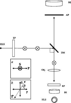

Fig. 7

Values of $M$ per pixel along an arbitrarily chosen straight line. On the left: average $M$ and SD values.

Fig. 8

Ten sequential measurements of $M$ for the same single pixel. The horizontal line represents the mean value of $M$ .

Appendix E: Microscope Adjustment for Fluorescence Polarization Measurements—a Short Review

The ever-increasing demand for microfluorometric, imaging-based FP measurements calls for a handy calibration procedure that would be most repeatable, accessible, easy to perform, integrative, and suitable for screening programs.

Generally, the optical arrangement required for correct FP measurements cannot be fully provided by microscopy. The reason for this is geometrical, deriving from the fact that in macrofluorometry both the excitation and the emission beams are presumably collimated $(NA \to 0)$ , which cannot be accomplished in microscopy. The higher the microscope objective’s numerical aperture, the larger the distortion of FP measurement.¹⁰ Hence, it appears that microscope standardization for FP measurements may have intrinsic limitations, independent of the calibration method used.

For the sake of brevity, let us consider the case of a microscopic cell, which is illuminated by a narrow excitation beam, having a considerably smaller radius than that of the objective lens (before impinging on it), and consequently remaining narrow and axial when illuminating the entire cell. Then (after taking into consideration all of the other “contributions”—see Appendix D—apart from NA dependence), it can be shown that the relation between the measured and true FP is given by:

Eq. 10

\frac{1}{P_{m}} = \frac{a (x)}{P} - b (x),

where

P_{m}

is the measured FP, which depends both on the true polarization

P

and on the objective angular aperture

X

. The coefficient

a

is bigger than

b

and both are constant for a given

X

. As

X

tends to 0, namely the more collimated the gathered illumination is,

P m \to P

.¹⁰

Actually, the quantity of interest is the relative change in $P m$ , that is $Δ P m ∕ P m$ (depolarization), which may be induced by biomodulating agents.

From Eq. 10, we obtain that $Δ P m ∕ P m$ is related to $Δ P ∕ P$ as:

Eq. 11

\frac{Δ P_{m}}{P_{m}} = [\frac{Δ P}{P}] {[1 - \frac{P b}{a}]}^{- 1} .

Thus, the percent change in the measured polarization depends not only on the true polarization percent change but also on the value of the true polarization itself.

According to Eqs. 10, 11, the higher the true polarization baseline, the greater the $Δ P m ∕ P m$ , even if considering the same $Δ P ∕ P$ values. For example, the change from $FP = 0.300$ to 0.330, and from 0.100 to 0.110, yield the same true $Δ P ∕ P$ of 10%. However, the measured change $Δ P m ∕ P m$ will be greater in the former case.

Since the true $P$ value of the microscopic object is unknown, the induced depolarization cannot be evaluated accurately. The most customary way out of such a situation is simply to lower the objective NA. By that means, $b (x) \to 0$ , $P m$ becomes proportional to $P$ , and consequently $Δ P m ∕ P m \to Δ P ∕ P$ . Unfortunately, this choice is not without its drawbacks, leading to a lower image resolution. Examples of this approach implementation can be found in the literature.²¹

The prior discussion leads to the frustrating conclusion that a precise determination of a microscopic object’s FP cannot be practically achieved by microscopy, and a compromise has to be reached.

Realistically speaking, this means that the investigator should recognize the FP range of the investigated sample, and adjust the measurement system (e.g., select the $M$ , NA, etc.), so that the measured FP changes will maximally reflect those of the true FP, or at least be proportional to them. In addition, not less importantly, the chosen calibration procedure should be maximally convenient, repeatable, integrative, and suitable for screening.

One of the procedures used to recover from microscope FP distortion is by using a drop of solution with known FP ( $\sim 100 μ m$ thick, flattened between the microscope slide and the cover glass), set in front of the objective. In the microscope, the collimated excitation beam is converged by the objective lens toward its focal point, where it diverges. This yields a cone-heading-cone fluorescent volume structure having a length equal to the fluorescent layer thickness. Consequently, the gathered fluorescence signal includes out-of-focus emission: originating above the focal point—with a higher NA, and that originating below it—with a NA lower than the NA of the objective. Thus, even though utilizing a single FP value drop, the gathered emission is actually an ensemble of unknown FPs. Clearly, the closer the fluorescent volume is to a point, the less serious the problem is, which may encourage the use of microscopic phantoms.

A microscopic object has a completely different fluorescence appearance from a fluorescent layer. For example, lymphocytes are spherical, about $7 μ m$ in diameter. Similarly, we may consider each fluorescence pixel in the image plane as a fluorescence point source. Hence, in microscopy, the measurement of FP of a microscopic fluorescent object differs from that of a homogeneous solution. Even if originally they may have the same FP, the two samples will yield different values. Consequently, calibrating the microscope with a drop of known polarization may accurately recover the known FP value for the solution sample, but not necessarily for the microscopic object.

In contrast, in macrofluorometry there is no distinction between measurements of homogeneous fluorescent solutions and diluted fluorescent cell suspensions. Generally speaking, in calibrating the microscope for fluorescence measurements, the greater the similarity of the phantom and the investigated object (in terms of dimensions, shape, etc.), the more correct is the calibration. The adoption of this rule is strongly recommended in microscopy-based FP measurements.

Along these lines, relating to the measurements of spherical cells, two microscopic phantoms are most feasible: the cells themselves and/or fluorescent microscopic beads. Yet, while intensity-calibrated beads are available, unfortunately there are no available FP-calibrated microscopic phantoms, to the best of our knowledge. Thus, the only way to measure the true FP of microscopic objects is when they are in ensemble, in a cuvette, using macrofluorometry. Assuming that each microscopic object has a single valued FP $(P_{j})$ , the ensemble $F P_{ensemble}$ is intensity averaged:

F P_{ensemble} = {[\frac{\sum {(I_{par})}_{j} - \sum {(I_{per})}_{j}}{\sum {(I_{par})}_{j} + \sum {(I_{per})}_{j}} = \frac{\sum {(I_{par} - I_{per})}_{j}}{\sum {(I_{par} + I_{per})}_{j}} = \frac{\sum {(I_{par} + I_{per})}_{j} \frac{{(I_{par} - I_{per})}_{j}}{{(I_{par} + I_{per})}_{j}}}{\sum {(I_{par} + I_{per})}_{j}}]}_{j = 1}^{j = n} = \frac{\sum_{j = 1}^{j = n} I_{j D} P_{j}}{\sum_{j = 1}^{j = n} I_{j D}} = \frac{\sum_{j = 1}^{j = n} I_{j D} P_{j}}{I_{T D}},

where

n

is the number of objects (emitters),

P_{j}

and

I_{j D}

are the FP and the detected fluorescence intensity (FI) of an object

j

,

I_{T D}

is the overall ensemble’s detected FI, and “par” and “per” denote parallel and perpendicular. Next, using a microscope, one can measure each object’s

P j

and

I_{j D}

, and subsequently can also calculate the intensity-averaged FP, integrating over the observed cells. Then, by equalizing the FPs obtained by macrofluorometry and microscopy, the

M

factor can be obtained. Even though this is a more correct procedure than using a drop of fluorescent solution, this type of approach does not fully address the need for pure microscopy-based microscopic object FP calibration, since it disregards the individual FP aspects of the objects.

Another approach is the use of capillary cuvettes mimicking cuvette-like microscopic objects²² containing a solution with a known FP (predetermined by macrofluorometry). Even though these procedures are very accurate and have a high research value in microfluorometry, they are lengthy and not user friendly, which prevents their use in screening programs. Moreover, the shelf-life of a filled capillary is very short due to fading, evaporation, etc., which makes it impractical for daily use.

Similarly, we found that the use of fluorescent beads, living/dead cells, and a variety of fluorescent solutions are far from addressing the need for a handy compromising calibration procedure described at the beginning of this appendix.

In particular, even though calibration by a drop of solution may be a suitable compromising remedy, it was found to be seriously limited with regard to several important practical aspects. The shelf-time of such microscopic phantoms is short, during which time the phantom’s own FP may change due to evaporation of the hosting medium, alteration in fluorophore concentration, variation of the optical pass through the sample, natural fading, etc. Alternatively, it has been attempted to store bulks of several different FP solutions and, when needed, prepare new fresh phantoms. Unfortunately, due to the practical inability to produce identical phantoms, very frequently, fresh phantoms from the same source yield different $M$ values.

The compromising procedure performed in the present study utilizes transmitted diffuse light from a halogen source of the microscope condenser (instead of a drop of solution). First, the characteristic zero polarization should be confirmed: all components (except for the condenser) including the analyzing polarizer (AP) and the emission detector (D2, see Fig. 6) were removed to allow direct measurement by the D2 (after passing through the AP). The constancy of the measured signal obtained in continuous rotation of the AP clearly attests to the zero polarization characteristic of the diffused halogen light. This is a once-a-year checkup and it is not considered a step in the measurement of $M$ , which is performed as follows (see Fig. 7).

Assuming that the AP is adjusted for the $S$ plane (normal to the plane of incidence $\otimes$ ) and the $P$ polarization plane (perpendicular to $S$ , vibrating in the plane of incidence $\leftrightarrow$ , see Fig. 6 insert), then $M$ simply equals the intensity ratio $I_{S} ∕ I_{P}$ of the condenser’s transmitted unpolarized light, after passing through all microscope components situated along its optical axis. This is a very user friendly procedure. All components needed for its performance are readily available, being an integrated part of the microscope system, thus even enabling the automation of this procedure. The legitimacy of this user friendly approach was carefully verified both by predetermined polarized light and FP solutions.

Predetermined Polarized Light

Here, the test microscope system comprises three polarizers: the emission polarizer (EP), analyzing polarizer (AP), and rotating polarizer (RP), which were meticulously adjusted, in the absence of the objective, as follows.

The collimated excitation beam, $S$ -polarized by the EP, impinges on the illuminator (dichotic mirror DM) at an incident angle of $45 \deg$ , is refracted at a right angle, and finally impinges upright on the RP surface computer-controlled rotating stepping motor, 20,000 steps per revolution). Next, the $S$ and $P$ polarization planes of the RP were carefully adjusted relative to the S polarized excitation beam (with the absence of the objective). Subsequently (after verifying the zero polarization of the diffused halogen light), the AP was adjusted (with the absence of the objective) for its corresponding $S$ and $P$ directions via the already adjusted RP, the condenser’s light, but in the absence of DM.

When the polarization angle of the RP was set at $45 \deg$ (between $S$ and $P$ ), the intensity components, $I_{S}$ parallel and $I_{P}$ perpendicular (measured by D2 after periodically setting the AP at $S$ and $P$ ), were found to be equal, hence they yield zero polarization (to the fourth decimal), again indicating zero polarization characteristic of the diffused halogen light. By this procedure, the system for predetermined polarized light measurements is prepared for use.

Next, the missing microscope components (e.g., DM, emission filters, objective, etc.) were reintroduced into the optical pass and, with the RP set at $45 \deg$ , $M$ $(= I_{S} ∕ I_{P})$ was predetermined and quite expectedly found (within the measurement system SD range) to be the same as measured with the absence of the RP (directly measuring the unpolarized light).

The $M$ suitability was then verified. The RP was set at a chosen angle $θ$ , the angle between the RP plane of polarization and the $S$ direction [see Fig. 6b]. Consequently, the true (theoretical) polarization of the light passing through the RP is:

p_{theory} = \frac{I_{S} - I_{p}}{I_{S} + I_{p}} = \frac{I_{0} \cos^{2} θ - I_{0} \sin^{2} θ}{I_{0} \cos^{2} θ + I_{0} \sin^{2} θ} = \cos^{2} θ - \sin^{2} θ = \cos 2 θ .

For each angle,

I_{S}

and

I_{P}

were analyzed by the AP and measured by the D2. The corresponding measured light polarization

P_{m}

(

m

denotes measured) was determined by the formula

P_{m} = [(I_{S} - M I_{P}) ∕ (I_{S} + M I_{P})]

. For each angle, 100 polarization measurements were performed. The relation between the theoretical and the actual measured polarization is illustrated in Fig. 9 .

Fig. 9

Theoretical polarization ( $P = \cos 2 θ$ left ordinate) versus measured polarization ${P_{m} = [(I_{S} - M I_{P}) ∕ (I_{S} + M I_{P})] - abscissa}$ , and the corresponding angles of polarization planes (right ordinate). Bars indicate SD.

Quality of $M$

The quality of $M$ determination by transmitted light was further reconfirmed by comparing the FP of dissolved fluorescein $(1 μ M)$ in glycerol-PBS solution, as measured by macrofluorometry and microfluorometry. In macrofluorometry, the sample was measured in a 1-cm cuvette, whereas in microscopy, a drop of the same solution was loaded on the microscope slide and covered by a cover glass. The sample height (optical pass) was determined by utilizing a heated and flattened parafilm (Pechinev, Plastic Packaging, Chicago,Illinois) sheet spacer ( $\sim 50 μ m$ height after heating andflattening).

The microfluorometric versus the macrofluorometric FP measurements, and the relevant glycerol concentrations are illustrated in Fig. 10 (from Ref. 6). Each solution was measured ten times in the fluorometer and 100 times using the microscope.

Fig. 10

Fluorescence polarization of $1 μ M$ fluorescein in glycerol-water solution measured by microfluorometry (left ordinate) and macrofluorometry (abscissa). Relevant glycerol concentrations are indicated (right ordinate). The figure is taken from Ref. 6.

The results shown in Figs. 9 and 10 clearly indicate that the $M$ value can be determined either by a drop of solution or by unpolarized transmitted light. Undoubtedly, the latter approach is much more user friendly.

Acknowledgments

This research was supported by the Horowitz Foundation.

References

1.

A. K. Kenworthy and M. Edidin, “Distribution of a glycosylphosphatidylinositol-anchored protein at the apical surface of MDCK cells examined at a resolution of

< 100 Å

using imaging fluorescence resonance energy transfer,” J. Cell Biol., 142 69 –84 (1998). https://doi.org/10.1083/jcb.142.1.69 0021-9525 Google Scholar

2.

A. K. Kenworthy, “Imaging protein-protein interactions using fluorescence resonance energy transfer microscopy,” Methods, 3 289 –296 (2001). 1046-2023 Google Scholar

3.

Z. Kam, T. Volberg, and B. Geiger, “Mapping of adherent junction components using microscopic resonance energy transfer imaging,” J. Cell. Sci., 108 1051 –1062 (1995). 0021-9533 Google Scholar

4.

A. L. Kindzelskii, W. Xue, R. F. Todd, and H. R. Petty, “Imaging the spatial distribution of membrane receptors during neutrophil phagocytosis,” J. Struct. Biol., 113 191 –198 (1994). 1047-8477 Google Scholar

5.

M. Elangovan, R. N. Day, and A. Periasamy, “Nanosecond fluorescence resonance energy transfer–fluorescence lifetime imaging microscopy to localize the protein interactions in a single living cell,” J. Microsc., 205 3 –14 (2002). https://doi.org/10.1046/j.0022-2720.2001.00984.x 0022-2720 Google Scholar

6.

M. Cohen-Kashi, S. Moshkov, N. Zurgil, and M. Deutsch, “Fluorescence resonance energy transfers measurements on cell surfaces via fluorescence polarization,” Biophys. J., 83 1395 –1402 (2002). 0006-3495 Google Scholar

7.

A. Periasamy, M. Elangovan, H. Wallrabe, J. N. Demas, M. Barroso, D. L. Brautigan, and R. N. Day, “Wide-field, confocal, two-photon and lifetime resonance energy transfer imaging microscopy,” Methods in Cellular Imaging, 295 –308 Oxford University Press, New York (2001). Google Scholar

8.

M. A. Rizzo and D. W. Piston, “A high contrast method for imaging FRET between fluorescent proteins,” Biophys. J., 88 L14-6 (2005). 0006-3495 Google Scholar

9.

A. Pope, U. Haupts, and K. Moore, “Homogeneous fluorescence readouts for miniaturized high-throughput screening: theory and practice,” Drug Discovery Today, 4 350 –362 (1999). 1359-6446 Google Scholar

10.

M. Deutsch, R. Tirosh, M. Kaufman, N. Zurgil, and A. Weinreb, “Fluorescence polarization as a functional parameter in monitoring living cells: theory and practice,” J. Fluoresc., 12 25 –44 (2002). 1053-0509 Google Scholar

11.

D. Fixler, R. Tirosh, N. Zurgil, and M. Deutsch, “Tracing apoptosis and stimulation in individual cells by fluorescence intensity and anisotropy decay,” J. Biomed. Opt., 10 034007 (2005). https://doi.org/10.1117/1.1924712 1083-3668 Google Scholar

12.

M. Shinitzky, Physiology of Membrane Fluidity, 2 –51 CRC Press, Boca Raton, FL (1984). Google Scholar

13.

S. Damjanovich, M. Edidin, J. Szollosi, and L. Tron, Mobility and Proximity in Biological Membranes, 2 –47 CRC Press, Boca1994). Google Scholar

14.

M. Shinitzky, Physiology of Membrane Fluidity, 176 –184 CRC Press, Boca Raton, FL (1984). Google Scholar

15.

S. I. Vavilov, “A theory of concentration quenching of fluorescence in solutions,” J. Phys. (USSR), 9 68 –76 (1945). 0368-3400 Google Scholar

16.

Vector Laboratories (Burlington, CA, (2005) Google Scholar

17.

F. A. Quiocho, G. N. Reeke, J. W. Becker, W. N. Lipscomb, and G. M. Edelman, “Structure of concanavalin A at

4 Å

resolution,” Proc. Natl. Acad. Sci. U.S.A., 68 1853 –1857 (1971). 0027-8424 Google Scholar

18.

S. Damjanovich, M. Edidin, J. Szollosi, and L. Tron, Mobility and Proximity in Biological Membranes, 49 –108 CRC Press, Boca Raton, FL (1994). Google Scholar

19.

I. A. Hemmila, Applications of Fluorescence in Immunoassays, 113 John Wiley and Sons, New York (1991). Google Scholar

20.

D. Fixler, Y. Yishay, and M. Deutsch, “Influence of fluorescence anisotropy on fluorescence intensity and lifetime measurement: Theory, simulations and experiments,” IEEE Trans. Biomed. Eng., 53 1141 –1152 (2006). 0018-9294 Google Scholar

21.

A. Squire, P. J. Verveer, O. Rocks, and P. I. Bastiaens, “Red-edge anisotropy microscopy enables dynamic imaging of homo-FRET between green fluorescent proteins in cells,” J. Struct. Biol., 147 62 –69 (2004). 1047-8477 Google Scholar

22.

M. Sernetz and A. Thaer, Fluorescence Techniques in Cell Biology, 41 –49 Springer Verlag, New York (1972). Google Scholar

Citation Download Citation

Meir Cohen-Kashi, Yaniv Namer, and Mordechai Deutsch "Fluorescence resonance energy transfer imaging via fluorescence polarization measurement," Journal of Biomedical Optics 11(3), 034015 (1 May 2006). https://doi.org/10.1117/1.2209955

Published: 1 May 2006

Access the abstract

JOURNAL ARTICLE
13 PAGES

DOWNLOAD PAPER SAVE TO MY LIBRARY

GET CITATION

CITATIONS

Cited by 8 scholarly publications.

Explore citations on Lens.org

RIGHTS & PERMISSIONS

Get copyright permission Get copyright permission on Copyright Marketplace

KEYWORDS

Polarization

Fluorescence resonance energy transfer

Luminescence

Microscopes

Image filtering

Objectives

Polarizers

1.

Introduction

Eq. 1

Eq. 2

2.

Material and Methods

2.1.

Cells

2.2.

Concanavalin A

2.3.

Cell Labeling

2.4.

Imaging Instrumentation

Fig. 1

2.5.

Data Acquisition

2.6.

Data Analysis

2.7.

Fluorescence Polarization Imaging

Eq. 3

2.8.

E Imaging

Eq. 4

3.

Results and Discussion

3.1.

Fluorescence Resonance Energy Transfer Imaging

Fig. 2

Table 1

Fig. 3

Table 2

Fig. 4

3.2.

Integrated Versus Filtered Image Analysis

Fig. 5

4.

Conclusion

Appendices

Appendix A: Determination of E by Polarization Measurement

Eq. 5

Eq. 6

Eq. 7

Eq. 8

Eq. 9

Appendix B: Evidence of Fluorescence Resonance Energy Transfer from ConA-F to ConA-R, and Assessment of E via Fluorescence Polarization Versus Fluorescence Intensity

Experiment 1: Demonstration of Fluorescence Polarization-Based Fluorescence Resonance Energy Transfer on Isolated Proteins in Solution

Experiment 2: Donor’s Fluorescence Polarization with Different Concentrations of the Acceptor

Table 3

Experiment 3: Comparison between E Values Determined by Fluorescence Polarization and Fluorescence Intensity Measurements

Table 4

Appendix C: Possible Measurement Distortion in Fluorescence Resonance Energy Transfer from Donor Fluorophore X to Acceptor Y

Table 5

Appendix D: The Origins of the Microscope Correction Factor M

Physical Origin

Definitions and Geometrical Aspects

Notes

Fig. 6

Fig. 7

Fig. 8

Appendix E: Microscope Adjustment for Fluorescence Polarization Measurements—a Short Review

Eq. 10

Eq. 11

Predetermined Polarized Light

Fig. 9

Quality of M

Fig. 10

Acknowledgments

References

Show All Keywords

Keywords/Phrases

Search In:

Publication Years

Appendix C: Possible Measurement Distortion in Fluorescence Resonance Energy Transfer from Donor Fluorophore $X$ to Acceptor $Y$

Appendix D: The Origins of the Microscope Correction Factor $M$

Quality of $M$