|
|
1.IntroductionSince the introduction of infrared as a dream beam,1 infrared spectroscopy has been applied for measuring blood glucose noninvasively. There have been even some premature announcements of a noninvasive glucose monitor in the market, but still hope for and doubts of this technology prevail without a commercial product available at this time. There have been many investigations, for example, from an early scientific investigation by Robinson 2 and several papers have reviewed this technology. 3, 4, 5, 6 Initial investigations for noninvasive glucose monitoring used a wavelength region of 700 to that contains higher orders of glucose overtone regions.2, 7, 8 However, this wavelength region shows very little glucose absorption, for example, less than 0.1%, compared to the fundamental absorption region of 9 to . Naturally, other glucose absorption regions were explored. They are the combination spectral region between 2.0 and and the first overtone band of 1.52 to . Based on the measurements at these bands, studies have been made with aqueous solutions mixed with some blood substances, 9, 10, 11, 12 with blood13, 14 and in vivo experiments.15, 16 The fundamental glucose absorption band lies in the mid-infrared (MIR) region. Due to interference with other substances, 9.0 and are expected to be the most promising wavelengths to predict glucose absorption in the MIR region when interferences by other blood substances are also taken into account.17 There have been various investigations on measuring glucose using the MIR region. 18, 19, 20, 21 Unfortunately, the MIR region may not be used for in vivo monitoring because light penetration is limited to only several scores of micrometers depending on specific wavelengths. The near-infrared (NIR) 1.5 to band appears to be a suitable region for noninvasive glucose monitoring because it has higher glucose sensitivity compared with the second or third overtones and deeper penetration compared with the fundamental region. Basically, difficulties lie principally in weak glucose absorption, strong light scattering, and the interferences by other blood substances as well as other tissues. Initial enthusiasm from successful experiments with cuvette samples was often replaced by frustration when researchers performed in vivo experiments. A powerful tool, multivariate analysis, such as partial least-squares regression, may convert spectra to glucose fitting erroneously according to temporal or environmental correlation.22, 23 Is it possible to achieve noninvasive glucose monitoring particularly using NIR absorption spectroscopy? What would be an order of achievable maximum accuracies? As one of the steps toward noninvasive glucose monitoring, whole blood samples were investigated in this study. Interestingly enough, there has been little investigation on glucose prediction using whole blood. Amerov used bovine blood from a single blood matrix.14 They had varied glucose concentrations. However, other blood components were the same. In our case, we used human whole blood. Our samples had different concentrations of glucose and hemoglobin as well as other blood substances. Because our research aim was to know how accurately blood glucose can be monitored, we used the different blood samples instead of a single matrix. Other human whole blood research that we are aware of was by Haaland 13 They prepared blood samples from only four persons. Twenty samples from each person were made. Predictions in terms of the standard error of prediction (SEP) using the samples made from the same person ranged from 30.5 to . However, predictions based on the calibration model using a different individual were poor and they did not even reveal the numbers. They stated that different blood compositions were sufficiently different among the four subjects. In our study, the number of different blood samples was increased so that different blood chemistry was taken into account. We examined which optimal wavelength regions should be used to predict glucose concentrations in the NIR region. We also studied the effect of data preprocessing and the influence of hemoglobin that is the most dominant component in blood. 2.ExperimentsA 6500 spectrometer equipped with silicon and lead-sulfide (PbS) detectors was used to measure the spectra of 98 blood samples. Each blood sample was made by pooling 3 to 5 EDTA whole blood samples where both blood types (ABO and Rh) and hemoglobin concentrations were being checked. Pooling blood was required to ensure that there was enough blood volume when preparing each sample that was used not only for spectrum measurement but also for reference value measurement. Glucose stock solution of in saline was added to blood samples to control glucose concentrations. Highly concentrated glucose stock was added into a different blood sample to make a blood sample with a particular glucose concentration. No dilution of blood was made. First, we had information on hemoglobin concentration for every extracted blood sample. We mixed (or pooled) 3 to 5 extracted blood samples of similar hemoglobin concentrations to make one blood sample. By doing this, we had enough blood volume for each sample. Also during this process, we could arrange the samples so that their hemoglobin concentrations were distributed in the entire physiological range. After that, we added glucose to assign different glucose values such that glucose and hemoglobin concentrations are not correlated to each other. Spectra were measured by a NIR 6500 system between and with a step of . One scan time was set to and 32 scan data were averaged to produce a spectrum. The system signal-to-noise ratio of measured spectrum was absorbance that was computed from two consecutively acquired spectra. Each spectrum was obtained between 1100 and . Whole blood was contained in a detachable cell. The spectrum of the blood sample was measured. The spectrum without the cell was also measured and used for reference. The absorbance spectrum was obtained from these two single beam intensities. Immediately after each measurement, a portion of blood was centrifuged and the plasma was frozen to measure glucose concentration. A chemistry analyzer based on the glucose hexokinase method was used to measure plasma glucose. Using another portion of the same blood, hemoglobin concentration was measured by the method using a instrument. Measured glucose and hemoglobin for 98 samples ranged from 45 to and 7.5 to , respectively. Figure 1a shows measured transmission spectra. Whole blood shows higher absorption than saline [see Fig. 1a]. In our figures, values around , a very strong water absorption peak, are not shown in order to increase the dynamic range of the axis. Correlation coefficients between hemoglobin or glucose values with respect to whole blood absorbance for all the samples were calculated at each wavelength. Correlation coefficients of hemoglobin and glucose with respect to absorbance at each wavelength are shown in Fig. 1b. Correlation coefficients for hemoglobin are around 0.8 and those for glucose are smaller than 0.1. This indicates that measured absorbance spectra varied mainly depending on hemoglobin level. Fig. 1(a) Whole blood spectra of 98 samples and saline spectrum; (b) whole blood spectra are correlated with hemoglobin and glucose concentrations at each wavelength and computed correlations coefficients are shown. 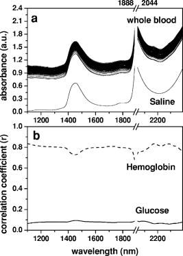 2.1.Wavelength SelectionThe region between 1100 and includes the first overtone and combination bands. It is necessary to choose a specific wavelength region that minimizes prediction errors. We performed partial least-squares regression (PLSR) analysis by using 2.6 software (Infometrix Inc). All 98 samples were examined. Before calibration, spectra were mean-centered. We used all the sample data. Loading vectors were analyzed to examine the influence of wavelength. Our previous work,24 has more detailed descriptions on loading vector analysis and wavelength band selections. A similar approach was adapted in this investigation. In choosing the wavelength ranges, a region between 1.5 and (first overtone band) and a region between approximately 2 to (combination band) were considered. Also, the entire range of 1.1 to was included as one of the regions. A region around has a higher water absorption peak and hemoglobin absorption increases toward . Therefore, the elimination of 1940 and peaks produced further wavelength regions (Table 1 ). Table 1 summarizes glucose prediction at various spectral regions. For each spectral region, we computed the standard error of cross validation (SECV), correlation coefficient of cross validation (rCVal), standard error of calibration (SEC), correlation coefficient of calibration (rCal), and coefficient of variation in cross validation . An optimum number of factors used in the regression were determined by the leave-one-out cross validation and test with a significance level of 5% among the factors. The best result was obtained using the regions of 1390 to 1888 and 2044 to where SECV is the least. Table 1Predictions of glucose concentrations at various spectral regions. Spectra of all 98 samples were used. The best SECV and VCCVal were obtained when 1390 to 1888 and 2044 to 2392nm were used.
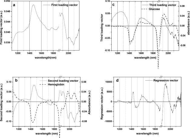
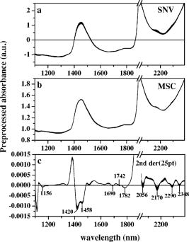
Over 1100 to , except for a water absorption peak around , we plotted the first through third loading vectors and regression vectors of a glucose calibration model that used all 98 samples (Fig. 2 ). Loading vectors are shown together with glucose spectrum [Fig. 2b] and hemoglobin spectrum [Fig. 2c] whose values were measured from saline solutions. Therefore, a spectrum of glucose or hemoglobin in Fig. 2 was calculated by subtracting saline spectra. Hemoglobin was prepared by the blood cell lysis method described in the Ref. 25. 2.2.Data Preprocessing and EnhancementVarious data preprocessing methods have been utilized to improve calibration and prediction modeling. In this study, multiplicative scatter correction (MSC)26 and standard normal variate (SNV)27 were tested in order to minimize the scattering effect of blood cells. In addition, the second derivative method that has been widely used to remove baseline variations was applied. Fifteen or 25 points smoothing was made before differentiation to reduce noises. After preprocessing, mean centering was applied for data enhancement. Figure 3 shows final spectra processed by MSC, SNV, and the second derivatives. In order to study the effect of preprocessing, glucose concentrations were predicted. In this case, we used the wavelength bands of 1390 to 1888 and 2044 to that produced the best results in Sec. 2.1. The results were summarized in terms of SECV and as shown in Table 2 . Table 2The effects of spectral data preprocessing in terms of SEC: all 98 samples were calibration modeled using different preprocessed spectra at the wavelengths of 1390 to 1888 and 2044 to 2392nm .
2.3.Influence of Hemoglobin LevelHemoglobin is the most dominant component in blood, and its concentration level is more than 100 times of glucose. Its absorbance becomes increasingly strong toward short NIR and visible wavelengths. Even though hemoglobin absorption peaks do not interfere with the peaks of other components, its influence is by no means negligible due to its high concentration.4, 17 Therefore, it is expected that calibration and prediction modeling can be substantially influenced by hemoglobin level. To study hemoglobin influence, 98 samples were divided into several groups. First, the entire samples were divided into two groups that are the calibration set (63 samples) and the prediction set (35 samples). Both groups were arranged so that hemoglobin and glucose concentrations were evenly distributed. Next, all the samples were grouped into three groups depending on hemoglobin level ( : 16.6 to ; : 12.8 to ; : 10.7 to ). Each of three groups had glucose concentrations evenly distributed in the entire range. Table 3 summarizes the groups, ranges of hemoglobin and glucose, and their standard deviations. It is important that hemoglobin and glucose concentrations in each group are not correlated. All five groups were checked for the correlation between hemoglobin and glucose concentrations, and we verified that the correlations were negligible as can be seen in terms of the correlation coefficient, (Table 3). Table 3Concentration distributions of hemoglobin and glucose in different sample groups.
Calibration modeling was performed using the four calibration groups ( , , , and ). Wavelength bands of 1390 to and 2044 to with mean centering were applied in PLSR analysis. The results were shown in Table 4 . Table 5 displays SEP and correlation coefficient of prediction . Because glucose values are different among the prediction sets, prediction accuracy was analyzed in terms of the coefficient of variation in prediction . is defined as (SEP/mean value of glucose) 100 expressed as a percentage. The results are summarized in Table 5. Table 4The result of calibration models for glucose determination from the four calibrations sets of different hemoglobin levels. PLSR was performed using the bands of 1390 to 1888 and 2044 to 2392nm with mean centering.
Table 5Prediction of glucose concentrations based on the four calibration models.
3.Results and DiscussionBefore further analysis of data preprocessing and hemoglobin influence, an optimal wavelength region that provided the least calibration errors was obtained. SECV varied widely between 26.1 and , while various wavelength regions in 1100 to were tested (Table 1). The best results were achieved when the regions of 1390 to and 2044 to were used. The regions contain both first overtone and combination bands. The optimal region included a water absorption peak at in the first overtone band, but excluded a water absorption peak of and wavelengths shorter than .28 As can be observed in Fig. 1a, the region between 1100 and shows different slopes between hemoglobin and glucose. Absorption of saline decreases as the wavelength becomes shorter. This is a typical feature of the water absorption spectrum. On the other hand, blood absorption increases toward . This reflects hemoglobin absorption. When 1100 to was included, SECV increased from to . Figure 2 shows loading vectors between 1100 and . The first loading vector appears to represent a spectral profile of blood to some degree [Fig. 2a]. The second loading vector is similar to hemoglobin spectrum, but it is a mirror image [Fig. 2b]. A spectral pattern of glucose looks similar to that of the third loading vector although there is a mismatch at wavelengths shorter than [Fig. 2c]. It is interesting to note that the exclusion of 1100 to produced better glucose prediction. Figure 2d illustrates regression vectors. The high absolute value of the regression vector indicates high contribution to glucose calibration at that wavelength. No contribution of 1100- is again observed in Fig. 2d. However, strong influences by two water absorption peaks (1440 and ) are depicted in Fig. 2. Applying scattering correction methods of MSC and SNV did not improve the prediction accuracy as can be seen in Table 2. Figure 3 shows preprocessed spectra by MSC, SNV, and second derivatives. In the case of the second derivative method that has been widely used for baseline correction, the results were the worst and produced higher numbers of factors. For the second derivatives, negative peaks appeared at 1420, 1458, 1690, 1742, 1782, 2056, 2170, 2290, and . Peaks at 1420 and belong to the water absorption band and the rest are close to the peaks in the second derivative spectra of hemoglobin (1690, 1740, 2056, 2170, 2290, and ) given by Kuenstner and Norris.25 This indicates that whole blood spectra are dominated by hemoglobin spectra. Hemoglobin features appear to be more enhanced than glucose features during differentiation. The influence of hemoglobin concentrations in the samples was summarized in Table 4. Calibration modeling using had SECV of and of 13.4%. When calibration models from the sets of high, medium, and low hemoglobin levels ( , , and , respectively) were performed, SECV ranged between 29 and and varied from 13.1 to 18.0%. Glucose concentrations were predicted and the results were summarized in Table 5. Based on the calibration model using 63 samples , glucose values of the other 35 samples were predicted. SEP was where the mean value of glucose was and was 11.2%. Cross predictions among the different groups of hemoglobin levels were made. SEPs varied a great deal depending on the groups. We observed SEPs of 23.1 to and of 10.8 to 22% (Table 5). The more difference in hemoglobin level between the sets, the higher prediction error appeared to be. For example, was 35.8% when was predicted based on the calibration model of . When the calibration model based on predicted glucose concentrations of , was 22%. The highest values were 35.8 and 22%. It is observed that hemoglobin distribution in the calibration or prediction model influenced the accuracy substantially. It is expected that the calibration model should use a sample set consisting of all physiological ranges for hemoglobin levels. 4.SummaryFirst overtone band or combination band alone was not a sufficient wavelength region in predicting glucose in whole blood. The region including both bands, but excluding a water absorption peak of , gave better prediction. A simple mean centering as a data preprocessing method produced good results in the optimal wavelength region. However, we may have to limit our statement to our particular case of PLSR analysis and whole blood samples because the generalization about preprocessing may be dependent on a particular multivariate method and samples. When whole blood was dealt with, hemoglobin concentrations in the calibration model should represent an entire range of hemoglobin. We have not found previous investigations where the actual hemoglobin concentrations were analyzed either for blood analysis or for in vivo experiment. We obtained a SEP of where blood glucose ranged between 45 and . The coefficient of variation in prediction was 11.2%. For noninvasive glucose monitoring, person-to-person blood chemistry as well as tissue variations make situations more difficult. When individual calibration (i.e., personal use) is adapted, the problem of person-to-person variation can be avoided. The personal calibration is recommended as a first step toward a noninvasive glucose monitor. AcknowledgmentsThis work was supported in part by the Ministry of Science and Technology of Korea through the Cavendish-KAIST Cooperative Research Program. We thank Haemin Cho for spectrum measurements. ReferencesI. Amato,
“Race quickens for non-stick blood monitoring technology,”
Science, 258 892
–893
(1992). 0036-8075 Google Scholar
M. R. Robinsons,
R. P. Eaton,
D. M. Haaland,
G. W. Koepp,
E. V. Thomas,
B. R. Stallard, and
P. L. Robinson,
“Noninvasive glucose monitoring in diabetic patients: A preliminary evaluation,”
Clin. Chem., 38
(9), 1618
–1622
(1992). 0009-9147 Google Scholar
H. M. Heise,
“Non-invasive monitoring of metabolites using near infrared spectroscopy: state of the art,”
Horm. Metab. Res., 28 527
–534
(1996). 0018-5043 Google Scholar
O. S. Khalil,
“Spectroscopic and clinical aspects of noninvasive glucose measurements,”
Clin. Chem., 45
(2), 165
–177
(1999). 0009-9147 Google Scholar
R. McNichols and
G. L. Cote,
“Optical glucose sensing in biological fluids: an overview,”
J. Biomed. Opt., 5
(1), 5
–16
(2000). https://doi.org/10.1117/1.429962 1083-3668 Google Scholar
A. Sieg,
R. H. Guy, and
M. B. Delgado-Charro,
“Noninvasive and minimally invasive methods for transdermal glucose monitoring,”
Diabetes Tech. Ther., 7
(1), 174
–197
(2005). Google Scholar
R. D. Rosenthal,
“Method for providing general calibration for near infrared instruments for measurement of blood glucose,”
(1993) Google Scholar
U. A. Muller,
B. Mertes,
C. Fischbacher,
K. U. Jageman, and
K. Danzer,
“Non-invasive blood glucose monitoring by means of near infrared spectroscopy: methods for improving the reliability of the calibration models,”
Int. J. Artif. Organs, 20
(5), 285
–290
(1997). 0391-3988 Google Scholar
M. R. Riley,
M. A. Arnold, and
D. W. Murhammer,
“Matrix-enhanced calibration procedure for multivariate calibration models with near-infrared spectra,”
Appl. Spectrosc., 52
(10), 1339
–1347
(1998). 0003-7028 Google Scholar
G. Yoon,
A. K. Amerov,
K. J. Jeon, and
Y.-J. Kim,
“Determination of glucose concentration in scattering medium using selected wavelengths at overtone absorption band,”
Appl. Opt., 41
(7), 1469
–1475
(2002). 0003-6935 Google Scholar
L. Zhang,
G. W. Small, and
M. A. Arnold,
“Multivariate calibration standardization across instruments for the determination of glucose by Fourier transform near-infrared spectroscopy,”
Anal. Chem., 75 5905
–5915
(2003). https://doi.org/10.1021/ac034495x 0003-2700 Google Scholar
J. Chen,
M. A. Arnold, and
G. W. Small,
“Comparison of combination and first overtone spectral regions for near-infrared calibration models for glucose and other biomolecules in aqueous solutions,”
Anal. Chem., 76 5405
–5413
(2004). 0003-2700 Google Scholar
D. M. Haaland,
M. R. Robinson,
G. W. Koepp,
E. V. Thomas, R. P. Eaton,
“Reagentless near-infrared determination of glucose in whole blood using multivariate calibration,”
Appl. Spectrosc., 46
(10), 1575
–1578
(1992). 0003-7028 Google Scholar
A. K. Amerov,
J. Chen,
G. W. Small, and
M. A. Arnold,
“Scattering and absorption effects in the determination of glucose in whole blood by near-infrared spectroscopy,”
Anal. Chem., 77 4587
–4594
(2005). 0003-2700 Google Scholar
J. J. Burmeister,
M. A. Arnold, and
G. W. Small,
“Noninvasive blood glucose measurements by near-infrared transmission spectroscopy across human tongues,”
Diabetes Tech. Ther., 2
(1), 5
–16
(2000). Google Scholar
K. Maruo,
M. Tsurugi,
J. Chin,
T. Ota,
H. Arimoto,
Y. Yamada,
M. Tamura,
M. Ishii, and
Y. Ozaki,
“Noninvasive blood glucose assay using a newly developed near-infrared system,”
IEEE J. Sel. Top. Quantum Electron., 9
(2), 322
–330
(2003). 1077-260X Google Scholar
H. Zeller,
P. Novak, and
R. Landgraf,
“Blood glucose measurement by infrared spectroscopy,”
Int. J. Artif. Organs, 12
(2), 129
–135
(1989). 0391-3988 Google Scholar
H. M. Heise,
R. Marbach,
G. Janatsch, and
J. D. Kruse-Jarres,
“Multivariate determination of glucose in whole blood by attenuated total reflection infrared spectroscopy,”
Anal. Chem., 61 2009
–2015
(1989). 0003-2700 Google Scholar
R. A. Shaw,
S. Kotowich,
M. Leroux, and
H. H. Mantsch,
“Multivariate serum analysis using mid-infrared spectroscopy,”
Ann. Clin. Biochem., 35 624
–632
(1998). 0004-5632 Google Scholar
S. Hahn,
G. Yoon,
G. Kim, and
S.-H. Park,
“Reagentless determination of human serum components using infrared absorption spectroscopy,”
J. Opt. Soc. Korea, 7
(4), 240
–244
(2003). Google Scholar
Y.-J. Kim,
S. Hahn, and
G. Yoon,
“Determination of glucose in whole blood samples by mid-infrared spectroscopy,”
Appl. Opt., 42
(4), 745
–749
(2003). https://doi.org/10.1038/nj6959-745a 0003-6935 Google Scholar
M. A. Arnold,
J. J. Burmeister, and
G. W. Small,
“Phantom glucose calibration models from stimulated noninvasive human near-infrared spectra,”
Anal. Chem., 70 1773
–1781
(1998). https://doi.org/10.1021/ac9710801 0003-2700 Google Scholar
R. Liu,
W. Chen,
X. Gu,
R. K. Wang, and
K. Xu,
“Chance correlation in non-invasive glucose measurement using near-infrared spectroscopy,”
J. Phys. D, 38 2675
–2681
(2005). 0022-3727 Google Scholar
Y.-J. Kim and
G. Yoon,
“Multicomponent assay for human serum using mid-infrared transmission spectroscopy based on component-optimized spectral region selected by first loading vector analysis,”
Appl. Spectrosc., 56
(5), 625
–632
(2002). https://doi.org/10.1366/0003702021955187 0003-7028 Google Scholar
J. T. Kuenstner and
K. H. Norris,
“Spectrophotometry of human hemoglobin in the near infrared region from 1000 to ,”
J. Near Infrared Spectrosc., 2 59
–65
(1994). Google Scholar
H. Martens and
T. Næs, Multivariate Calibration, John Wiley & Sons Ltd., New York (1989). Google Scholar
M. S. Dhanoa,
S. J. Lister,
R. Sanderson, and
R. J. Barnes,
“The link between multiplicative scatter correction (MSC) and standard normal variate (SNV) transformations of NIR spectra,”
J. Near Infrared Spectrosc., 2 43
–47
(1994). Google Scholar
G. M. Hale and
M. R. Querry,
“Optical constants of water in the 200-nm to wavelength region,”
Appl. Opt., 12
(3), 555
–563
(1973). https://doi.org/10.1007/BF00934777 0003-6935 Google Scholar
|