2.1.

The Phantom Using Point Illumination/Point Collection Geometry

In this study, image reconstructions were performed using measured fluorescent light intensity and phase-shift acquired on the surface of a breast-shaped phantom as shown in Fig. 1 . The hemispherical portion of the phantom (10-cm diameter) represents the breast tissue and the cylindrical portion (20-cm diameter and 2.5-cm height) represents the extended chest wall regions. Point illumination and point collection geometry was used to acquire data using optical fibers of 1-mm diameter that were located in concentric rings along the hemispherical surface of the phantom. The tissue phantom was filled with a 1% Liposyn solution to mimic the scattering properties of tissue. Different spherical target volumes (0.5 and $1.0{\mathrm{cm}}^3$ ) were filled with the 1% lipid containing $1\mathrm{\mu }\mathrm{M}$ Indocyanine Green as the fluorophore. The targets were placed $1.4–2.8\mathrm{cm}$ deep within the phantom (for further details on the phantom and measurement geometry, see Refs. 30, 31, 32). The optical properties of the background and targets used in these experiments are given in Table 1 . In experiments #1–7, $1\mathrm{\mu }\mathrm{M}$ ICG was used in the spherical target while in experiment #8, three $\sim 0.5\mathrm{cc}$ spherical targets containing $2.5\mathrm{\mu }\mathrm{M}$ ICG were positioned within the background containing no ICG.

Fig. 1

Schematic showing point illumination and point collection of a breast-shaped phantom with the cup-shaped portion (10-cm diameter) representing the breast tissue, and the cylindrical portion (20-cm diameter and 2.5-cm height) representing the extended chest wall region around the breast. Phantom set-up including collection fibers that are interfaced to the hemispherical surface of the phantom on one end, and to either of two interfacing plates on the other end.

Table 1

Optical properties of target and surroundings in perfect and imperfect data measurement sets.

2.2.

Measurement Approach

Time-dependent emission measurements reflecting light propagation and decay kinetics were made using frequency-domain techniques. The phantom was sequentially illuminated at a single point on the phantom surface with intensity modulated excitation light ( $783\mathrm{nm}$ at $100\mathrm{MHz}$ modulation frequency) using $1000\text{-}\mathrm{\mu }\mathrm{m}$ diameter fiber optics to deliver excitation light. The fluorescent signal $\left(830\mathrm{nm}\right)$ was collected from point locations on phantom surface via $1000\text{-}\mathrm{\mu }\mathrm{m}$ diameter optical fibers. Interference $\left(830\mathrm{nm}\right)$ and holographic filters were used to block the excitation light. The light emitted from the ends of all collecting fibers were simultaneously collected using a gain-modulated intensified charge coupled device (ICCD) camera that was operated in homodyne mode. That is, the ICCD camera was used for simultaneous data acquisition from multiple collection fibers that were interfaced as 2-D arrays onto an interfacing plate to collect emission AC intensity $I_{A{C}_m}$ and emission phase-shift ${\theta }_m$ . Fluorescent measurements were acquired following illumination at single points, where the data used for reconstruction had an average fluorescent modulation depth (AC/DC) greater than 0.1.

2.3.

Imaging Trials Conducted

Experiments were conducted under different experimental conditions in which the fluorescent contrast of the target to background ratio (Target:Background=T:B) was either 1:0 or 100:1. In the case of perfect uptake (T:B=1:0), the objective was to detect fluorescent targets in an otherwise nonfluorescent background as may be the case for sentinel lymph node mapping. Here the fluorescent contrast agent may be injected peritumorally for uptake and mapping of the lymph flow to the major nodes in the body, and the background is essentially nonfluorescent. In the case of imperfect uptake (T:B=100:1), the objective was to mimic the optical contrast for systemically administered, molecularly targeting fluorescent contrast agents. When systemically administered, the agent is typically distributed in the background as well as within the target. We initially employ an optimal T:B ratio of 100:1 due to experimental limitations described ahead in the Discussion section.

Measurements were performed with a single spherical target of $0.5{\mathrm{cm}}^3$ or $1.0{\mathrm{cm}}^3$ volume at depths ranging from 1.4 to $2.8\mathrm{cm}$ from the phantom surface (based upon the centroid of the target). Measurements were also performed with multiple spherical targets of $0.5–0.6{\mathrm{cm}}^3$ volumes at approximately 1.4-cm distance from the phantom surface. In summary, eight experiments were conducted for tomographic reconstruction as described in Tables 1, 2 . The number of fluorescence intensity $I_{A{C}_m}$ and phase shift ${\theta }_m$ measurements made on the surface of the phantom for image reconstruction from each experiment are also given in Table 2.

Table 2

Experimental conditions, number of targets, location of targets, number of experimental measurements, relative model mismatch error of amplitude (EIAc) phase-shift (Eθ) , and number of unknowns of the inverse problems using Mesh 1 (coarse mesh) and Mesh 2 (fine mesh).

A reference scheme was used in this experimental data to reduce the instrument effects and the unknown source strength.^{24, 33} In the reference scheme, the emission fluences, ${\Phi }_m$ , from multiple collection fiber locations were referenced with respect to the emission fluence data from a single specified reference collection fiber $\left(ref\right)$ as given in Eq. 1:

2.4.

The Forward Problem to Predict Intensity $\left(I_{AC}\right)$ and Phase-Shift $\left(\theta \right)$ on Boundary Points

The diffusely propagated fluorescence in response to excitation illumination is predicted by the coupled diffusion Eqs. 2, 3:

2.5.

Formulation for Image Reconstruction

The starting point for formulating the reconstruction as an optimization problem begins with defining the error function $E({\mu }_{a_{xf}},\omega )$ ,

In the inverse problem, the selection of the error function [as given by Eq. 5] is important, because it determines how the measurements are related to the model. The fluence, ${\Phi }_m=I_{AC}{e}^{i\theta }$ , has been chosen because it contains all the available information and can be related to the observable measurements of amplitude intensity, $I_{AC}$ , and phase shift, $\theta$ . Since absolute measurements are not practical to acquire due to instrumentation effects and inability to calibrate each source, the measurement data and the calculated fluence were normalized as given in Eq. 1. The error function provides the difference between the normalized measurement and normalized computed fluence. We take the difference of the log of measured and computed normalized values since it results in a difference in phase and ratio of amplitude. We find this approch most effective. Since comparison of the difference of two complex values is difficult to translate into any physical meaning, the complex conjugate is introduced in Eq. 5 to ensure the error function is a real-valued norm.

The constrained truncated Newton with trust region (CONTN) method^{35, 36} and the nonlinear conjugate method were used to optimize the error function [Eq. 5] using the measured data. While target reconstructions were obtained using simulated data,^{35, 36} these methods failed to reconstruct targets when using experimental data. The most popular method for illconditioned problems is to use Tikhonov’s regularization technique.³⁷ The difficult and time-consuming task in Tikhonov regularization is to find the value of the regularization parameter given ground truth, something which is not available in true imaging situations. Hence, the PMBF/CONTN method was developed as described in Ref. 28. A brief description is contained in the following:

In the PMBF method, we use the modified barrier penalty function, $M$ (termed hereafter as the barrier function), to incorporate the constraints directly within the optimization variable: ^{28, 38, 39, 40}

The PMBF method is performed in two stages within an inner and an outer iteration. The outer iteration updates the Lagrange multiplier, $\lambda$ . Formulations used to update these parameters at each outer iteration are provided in Ref. 28. Using the calculated values of the parameters $\lambda$ and $f$ , CONTN is applied to minimize the penalty barrier function described by Eq. 7. Once satisfactory convergence within the inner iteration reached, the Lagrange multipliers, $\lambda$ , and the barrier parameter, $\eta$ , are updated in outer iteration and another constrained optimization is started within the inner iteration. A precise description on the PMBF/CONTN algorithm is provided in Ref. 28. Herein we also use the modified method of Breitfeld and Shanno³⁹ for initializing the Lagrange multipliers without a priori information. This effectively removes the need to choose an appropriate initial values of the Lagrange multipliers based upon ground truth, which in actual imaging is not known. The success of the algorithm depends upon the consistent convergence of both inner and outer iteration loops.

2.6.

Evaluation of Reconstructed Images

3.1.

Model Mismatch Error

The number of measurements in which the relative model mismatch errors of fluorescent amplitude $\left(E_{I_{AC}}\right)$ and phase shift $\left(E_{\theta }\right)$ were greater than 50% is given in Table 2. In all the experiments, the relative model mismatch errors of the amplitude are lower than that of phase shift. From Table 2, it can be seen that

Fig. 2

Histogram of relative model mismatch error, $E_{I_{AC}}$ , defined by Eq. 8 of fluorescence reference intensity $I_{A{C}_{ref}}$ for experiment #1.

Fig. 3

Histogram of relative model mismatch error, $E_{\theta }$ , defined by Eq. 9 of fluorescence reference phase-shift ${\theta }_{ref}$ for experiment #1.

3.2.

Target Depth Study (Single Spherical $\mathit{1}\text{-}{\mathit{cm}}^{\mathit{3}}$ Target)

The absorption coefficient due to the fluorescent, ${\mu }_{a_{xf}}$ , was reconstructed for the experiments $\#1–6$ . Figure 4 illustrates the PMBF/CONTN recovery of absorption coefficient due to fluorescence from referenced fluorescent measurements in experiment $\#1$ made under perfect uptake conditions. Similar imaging results were obtained for experiments $\#2–6$ for brevity, results are not shown. Tables 3, 4 summarize all the computed runs of experiments $\#1–6$ . In this set of reconstructions, the lower and the upper bounds were chosen to be $0.003{\mathrm{cm}}^{-1}$ and $0.3{\mathrm{cm}}^{-1}$ , respectively. Since the known amount of fluorophore was introduced, we can specify a lower bound greater than zero, and an upper bound of some practical value. Figure 4a represents the actual spatial distribution of fluorescence absorption coefficient, ${\mu }_{a_{xf}}$ , in $Z=2.4\text{-}\mathrm{cm}$ plane through the target when a target centroid of volume $1.0{\mathrm{m}}^3$ was located at $0.5$ , $-2.5$ , and $2.5\mathrm{cm}$ away from the surface (experiment #1) while Fig. 4b shows the reconstructed target in $Z=2.4\text{-}\mathrm{cm}$ plane through the target using an initial guess of uniform ${\mu }_{a_{xf}}^0$ to be $0.003{\mathrm{cm}}^{-1}$ and the initial Lagrange multipliers set to ${\lambda }_i^0=1000$ for perfect uptake condition. The reconstructed targets using the initial Lagrange multiplier set to ${\lambda }_i^0=1$ , 10, and 100 were identifiable (for brevity data not shown) but were consistently smaller in size than the actual target. In addition, the locations of the targets were shifted from the actual target position toward the illumination surface without the reconstruction of artifacts. Our results were the same with different initial values of ${\mu }_{a_{xf}}^0$ , if of course the initial values of ${\mu }_{a_{xf}}^0$ were chosen between the lower and upper bounds. To choose an initial value that violates these bounds violates the physics of the problem. Figure 4c shows the reconstructed target in $Z=2.4\text{-}\mathrm{cm}$ plane using the initial value of ${\lambda }_i^0$ computed using the method of Breitfeld and Shanno.³⁹ It is seen from Fig. 4 that the reconstructed targets are clearly identifiable and the shapes of the reconstructed targets are slightly larger than the true target. Similar trends were observed for other experiments as given in Tables 3, 4. Nonetheless it is found that it was not necessary to find the initial values of the Lagrange multiplier ${\lambda }_i^0$ by comparison with ground truth on a trial-and-error basis; but instead we could use the simple least-squares procedure to compute these values. Similar phenomena were observed when this reconstruction algorithm was applied to a phantom study using area illumination/collection geometry.²⁸

Fig. 4

Distribution of absorption coefficient due to fluorophore ${\mu }_{a_{xf}}{\mathrm{cm}}^{-1}$ with $1.0{\mathrm{cm}}^3$ spherical target located at $1.4\mathrm{cm}$ deep from the surface (centroid, 0.5, $-2.5$ , 2.5) under perfect uptake condition at $Z=2.4\text{-}\mathrm{cm}$ plane through the target, (a) actual distribution of the absorption coefficient due to fluorophore, (b) reconstructed image using initial value ${\mu }_{a_{xf}}^0=0.003{\mathrm{cm}}^{-1}$ and ${\lambda }^0=1000$ , (c) reconstructed image using initial value ${\mu }_{a_{xf}}^0=0.003{\mathrm{cm}}^{-1}$ and calculated ${\lambda }^0$ (experiment #1, Mesh 1).

Table 3

Summary of figures of targets reconstruction, CPU time and the root mean square error (RMSE) as a function of initial value of the absorption coefficient due to fluorophore μaxf0=0.003 and the initial Lagrange multiplier λ0=1000 as well as calculated λ0 (Ref. 28) for perfect and imperfect uptake measurement (experiments #1–4) using Mesh 1.

Table 4

Summary of figures of targets reconstruction, CPU time, and the root mean square error (RMSE) as a function of initial value of the absorption coefficient due to fluorophore μaxf0=0.003 and 0.002cm−1 and the initial Lagrange multiplier λ0=1000 as well as calculated λ0 (Ref. 28) for perfect and imperfect uptake measurements (Experiments #5–6) using Mesh 1 and Mesh 2.

Ten inner iterations and 10 outer iterations were required to reconstruct these images. The reconstructed images did not improve when we increased the number of inner iterations to 20 and outer iterations to 20. The total CPU time required with the different initial values of the Lagrange multipliers are given in Tables 3, 4. It can be seen that less CPU was required when the initial Lagrange multipliers were chosen to be, ${\lambda }^0=1000$ than when the values of ${\lambda }^0$ were calculated.

For quantitative analysis of the reconstructed images, values of the RMSE are listed in Tables 3, 4. The RMSE values are small when the initial Lagrange multipliers were chosen to be ${\lambda }^0=1000$ . The RSME values improved further when the initial Lagrange multipliers were calculated. Estimation of the target centriod with respect to the true centriod is tabulated in Tables 3, 4. The targets were reconstructed close to their true locations with no artifacts as shown in Fig. 4. In the cases of the perfect or imperfect experiments, the reconstructed depth targets were not underestimated as depth of the target increased from $1\mathrm{cm}$ to $2.8\mathrm{cm}$ .

These figures show that the PMBF/CONTN method is stable and accurate given the number of iterations required. The inner iteration is completed when the value of the barrier function is very small and further decrease is not possible. To summarize, the PMBF method with simple bounds on the optical properties of the tissue provides fast access to image recovery.

It is seen from Fig. 4 that the reconstructed targets are at the “true” location but larger in size. This may be due to large mesh sizes. To investigate this, a finer mesh (Mesh 2) was used. Figure 5 shows the recovery of absorption coefficient due to fluorophore by the PMBF/CONTN algorithm using the measurement data of experiment #5, i.e., a $10\text{-}{\mathrm{cm}}^3$ spherical target embedded $2.8\mathrm{cm}$ deep (centroid 0.5, $-1.5$ , 1.5). Figure 5a shows the true distribution of the absorption coefficient due to fluorophore in $Z=1.4\text{-}\mathrm{cm}$ plane through the target while Fig. 5b is the reconstructed images in $Z=1.4\text{-}\mathrm{cm}$ plane through the target using the initial Lagrange multiplier ${\lambda }^0=1000$ . Figure 5c is reconstructed in $Z=1.4\text{-}\mathrm{cm}$ plane through the target using the initial Lagrange multipliers ${\lambda }^0$ computed using the method of Breitfeld and Shanno.³⁹ The quantitative measures associated with the reconstructed images are listed in Tables 3, 4. It is seen in Tables 3, 4 that the volume of the reconstructed target is smaller in the fine mesh than that of coarse mesh. The volumes of the constructed targets are larger than the true volumes under conditions of imperfect uptake. Thus, the results show that a finer mesh provides a reconstructed volume closer to the actual volume. However, it is seen from Figs. 4 and 5 that the locations of the reconstructed images using both fine and coarse the finte element meshes are at the same locations as ground truth. As before, the centroids of the reconstructed targets using finer mesh are close to their true locations as given in Table 4. The maximum values of the absorption coefficients due to fluorophore in the reconstructed targets region and the true values are given in Tables 3, 4, which show that these values are closer to true values when a fine mesh used. The RSME using the fine mesh was slightly less than that of coarse mesh. Time required to reconstruct a target at $2.8\mathrm{cm}$ deep using the computed Lagrange multipliers on the Mesh 2 was $3\mathrm{hr}$ $50\min$ and on Mesh 1 was $45\min$ (Tables 3, 4). The time required to reconstruct the same sized target placed at $2\mathrm{cm}$ deep using the computed Lagrange multiplier on Mesh 2 was $2\mathrm{hr}$ $50\min$ while on Mesh 1 it took $29\min$ . Thus we see that the CPU time required for target reconstruction increases as the number of measurements increases, the target becomes deeper, and the mesh more refined.

Fig. 5

Distribution of absorption coefficient due to fluorophore ${\mu }_{a_{xf}}{\mathrm{cm}}^{-1}$ with $1.0{\mathrm{cm}}^3$ spherical target located at $2.8\mathrm{cm}$ deep (centroid 0.5, $-1.5$ , 1.5) under perfect uptake condition at $Z=1.4\text{-}\mathrm{cm}$ plane through the target, (a) actual distribution of the absorption coefficient due to fluorophore, (b) reconstructed image using initial value ${\mu }_{a_{xf}}^0=0.003{\mathrm{cm}}^{-1}$ and ${\lambda }^0=1000$ , (c) reconstructed image using initial value ${\mu }_{a_{xf}}^0=0.003{\mathrm{cm}}^{-1}$ and calculated ${\lambda }^0$ (experiment #5, Mesh 2).

We have demonstrated that the PMBF/CONTN reconstructed the targets accurately when the lower bound and the upper bounds of the absorption coefficient due to fluorophore, ${\mu }_{a_{xf}}$ , were 0.003 and $0.3{\mathrm{cm}}^{-1}$ , respectively, and the initial value of ${\mu }_{a_{xf}}$ were between the lower and upper bounds. In order to investigate the influence of the lower and upper bounds on the performance of the algorithm PMBF/CONTN, the lower bound and the upper bound of ${\mu }_{a_{xf}}$ , were chosen to be $0.002{\mathrm{cm}}^{-1}$ and $0.4{\mathrm{cm}}^{-1}$ , respectively, and the initial values of ${\mu }_{a_{xf}}$ were between these bounds. Figure 6 illustrates the recovery of absorption coefficient due to fluorophore by the PMBF/CONTN algorithm using the measurement data of experiment #6, i.e., a $1.0\text{-}{\mathrm{cm}}^3$ spherical target embedded in $2.8\mathrm{cm}$ deep (centroid 0.5, $-1.5$ , 1.5) under imperfect uptake. Figure 6a shows the actual distribution of the absorption coefficient due to fluorophore in $Z=1.4\text{-}\mathrm{cm}$ plane through the target. Figure 6b demonstrates the reconstructed target in $Z=1.4\text{-}\mathrm{cm}$ plane through the target using an initial guess of uniform ${\mu }_{a_{xf}}^0$ to be $0.002{\mathrm{cm}}^{-1}$ and the initial Lagrange multiplier ${\lambda }^0$ calculated by the modified method of Breitfeld and Shanno³⁹ (results of experiment #1 using the same lower and upper bounds are given in Table 3). The CPU time required for both these cases and the RMSE, location, and size of the target are nearly the same (Tables 3, 4). Thus we have seen the efficiency and accuracy of the PMBF/CONTN algorithm do not depend on the values of the lower and upper bounds providing these values based on physical considerations.

Fig. 6

Distribution of absorption coefficient due to fluorophore ${\mu }_{a_{xf}}{\mathrm{cm}}^{-1}$ with $1.0{\mathrm{cm}}^3$ spherical target located at $2.8\mathrm{cm}$ deep (centroid 0.5, $-1.5$ , 1.5) from the surface under imperfect uptake condition at $Z=1.4\text{-}\mathrm{cm}$ plane through the target, (a) actual distribution of the absorption coefficient due to fluorophore, (b) reconstructed image using initial value ${\mu }_{a_{xf}}^0=0.002{\mathrm{cm}}^{-1}$ and calculated ${\lambda }^0$ (experiment #6, Mesh 1).

In summary, the target depth studies demonstrated the capability of the algorithm to accurately detect single $1.0\text{-}{\mathrm{cm}}^3$ spherical targets located up to $2.8\mathrm{cm}$ deep under both perfect and imperfect conditions.

3.3.

Small Target Reconstruction (Single and Multiple Spherical Targets)

The absorption coefficient due to the fluorescent ${\mu }_{a_{xf}}$ was reconstructed for experiments $\#7–8$ . Figure 7 illustrates in plane through $Z=2.4$ , the PMBF recovery of absorption coefficient due to fluorophore from referenced fluorescent measurements made under perfect uptake conditions for experiment #8 (similar results were obtained using experiment #7). Table 5 summarizes all the computed runs of experiments $\#7–8$ . Figure 7a corresponds to the actual spatial distribution of fluorescence absorption coefficient, ${\mu }_{a_{xf}}$ , when multiple spherical targets of volume $\sim 0.55{\mathrm{cm}}^3$ were placed $1.4\mathrm{cm}$ away from the surface. Figure 7b demonstrates the reconstructed target using an initial guess of uniform ${\mu }_{a_{xf}}^0$ to be $0.003{\mathrm{cm}}^{-1}$ and the initial Lagrange multipliers chosen to be ${\lambda }_i^0=1000$ . As before, we also found that the initial Lagrange multiplier of ${\lambda }_i^0=1$ , 10, and 100 resulted in smaller target sizes and displaced reconstructed targets locations without artifacts. Figure 7c shows the reconstructed targets using the computed value of ${\lambda }_i^0$ . These results were obtained using Mesh 1. In each case the reconstructed single and multiple targets were clearly distinguishable from surroundings without artificats and the sizes of the reconstructed targets were smaller than the true targets. The centroid of the reconstructed targets and the actual location of the targets are given in Table 5. However, the targets were reconstructed close to their actual location with no artifcats as shown in Fig. 7.

Fig. 7

Distribution of absorption coefficient due to fluorophore ${\mu }_{a_{xf}}{\mathrm{cm}}^{-1}$ , three spherical targets of volumes $0.5–0.6{\mathrm{cm}}^3$ located $1.2–1.4\mathrm{cm}$ deep from the surface (centroids, $-1.0\text{,}-3.0$ , 1.8; $-1.0,2.0,2.9$ ; 2.0, $-1.0$ , 3.0) under perfect uptake condition at $Z=2.4\text{-}\mathrm{cm}$ plane through the targets, (a) actual distribution of the absorption coefficient due to fluorophore, (b) reconstructed image using initial value ${\mu }_{a_{xf}}^0=0.003{\mathrm{cm}}^{-1}$ and ${\lambda }^0=1000$ , (c) reconstructed image using initial value ${\mu }_{a_{xf}}^0=0.003{\mathrm{cm}}^{-1}$ and calculated ${\lambda }^0$ (experiment #8, Mesh 1).

Table 5

Summary of figures of targets reconstruction, CPU time, and the root mean square error (RMSE) as a function of initial value of the absorption coefficient due to fluorophore μaxf0=0.003cm−1 and the initial Lagrange multiplier λ0=1000 as well as calculated λ0 (Ref. 28) for perfect uptake measurements (Experiments #7–8) using Mesh 1 and Mesh 2.

As before, we also used the fine mesh (Mesh 2) for image reconstruction. Figure 8 shows the recovery of absorption coefficients ${\mu }_{a_{xf}}$ of three targets in plane through $Z=2.4$ . Figure 8a shows the true distribution of the absorption coefficient due to fluorophore while Fig. 8b illustrates the reconstructed targets using the initial Lagrange multiplier of ${\lambda }^0=1000$ . Figure 8c was reconstructed using the computed ${\lambda }^0$ . It is seen that the volume of the reconstructed targets in the fine mesh slightly smaller than that of coarse mesh (Table 5). Hence the results show that a finer mesh provides a reconstructed volume closer to the actual volume. They also show that the maximum absorption coefficients in the target region are slightly smaller using the fine mesh rather than the coarse mesh. That is, the reconstructed values are closer to the true values as the mesh was refined. This shows that we need finer meshes as the depth of the target increase. However, the locations of the reconstructed images using both the finite element meshes were at the same locations as the true images. The RSME using the fine mesh was slightly less than that of the coarse mesh (Table 5). Again, more CPU time was required when the initial value of ${\lambda }^0$ were calculated (Table 5). However, it should be noted that the overall CPU times could be higher if the trial-and-error method to find the Lagrange multipliers was used.

Fig. 8

Distribution of absorption coefficient due to fluorophore ${\mu }_{a_{xf}}{\mathrm{cm}}^{-1}$ , three spherical targets of volumes $0.5–0.6{\mathrm{cm}}^3$ located $1.2–1.4\mathrm{cm}$ deep from the surface (centroids, $-1.0\text{,}-3.0\text{,}1.8$ ; $-1.0,2.0,2.9$ ; 2.0, $-1.0\text{,}3.0$ ) under perfect uptake condition at $Z=2.4\text{-}\mathrm{cm}$ plane through the targets, (a) actual distribution of the absorption coefficient due to fluorophore, (b) reconstructed image using initial value ${\mu }_{a_{xf}}^0=0.003{\mathrm{cm}}^{-1}$ and ${\lambda }^0=1000$ , (c) reconstructed image using initial value ${\mu }_{a_{xf}}^0=0.003{\mathrm{cm}}^{-1}$ and calculated ${\lambda }^0$ (experiment #8, Mesh 2).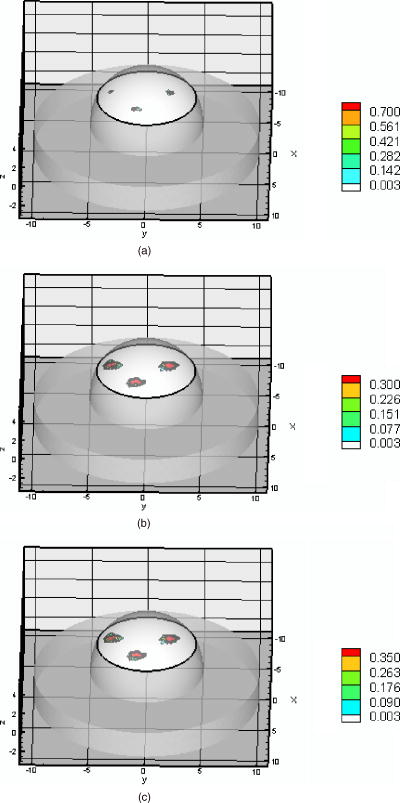

Both PMBF/CONTN and a Bayesian approach (AEKF)⁴¹ were used for the breast-shaped phantom studies. The referenced fluorescence measurement of intensity and phase shift were used in both algorithms to find the 3-D map of absorption coefficient due to fluorophore in the interior of the phantom. Details of the Bayesian method have presented elsewhere.⁴¹ To compare the performance of both algorithms, we have calculated the volumes of the reconstructed targets and found the centroid locations of the reconstructed targets. Results of experiments #2, 4, 6, and 8 using AEKF are discussed in Ref. 41. It was found that the reconstructed image using the AEKF was slightly shifted from the original location (Table 3 in Ref. 41) while the PMBF/CONTN reconstructed the images at the close to actual location as given in Table 6 . It was found that the AEKF underestimated the actual depth of the target as the depth increases.⁴¹ It was stated in Ref. 41 that the volume of the reconstructed target was sensitive to the threshold value of the reconstructed parameter and the threshold values were problem-dependent. The threshold value obtained for each experimental data has no mathematical foundation and was found from ground truth. A minimum-variance approach is used in the AEKF method. In this method the measurement error covariance and dynamically estimated parameter error covariance are used for the regularization of the ill-conditioned problem. While in the PMBF/CONTN method, the barrier and Lagrange multipliers regularize the solution. The PMBF method will converge, providing the Lagrange multipliers are positive.³⁸ Furthermore, an active constrained optimization method is utilized. In this method we divide the optimization variables in three parts based upon their local gradients, and accordingly these variables satisfy the lower and the upper bounds conditions.²⁸ Hence there is no threshold required. We have seen that volumes of the reconstructed images are slightly higher than the actual volume using a coarse mesh (Mesh 1), but the volumes reduced considerably when a fine mesh (Mesh 2) was used.

Table 6

Targets centroids and volumes calculated by PMBF/CONTN and AEKF.

Figures 3–5 in Ref. 41 showed there are some artifact effects using the experiments data specifically for imperfect uptake (T:B ratio, 100:1) with $10{\mathrm{cm}}^3$ spherical target located 2.04 and $2.82\mathrm{cm}$ deep. The artifacts increase as the depth of the target increases. We have seen in Figs. 6 and 7 in Ref. 41 that the artifacts were very high when three targets were reconstructed while the PMBF method reconstructed images without artifacts as shown in Figures 4, 5, 6, 7, 8.

To summarize, we have demonstrated that the algorithm based on the PMBF method with constrained optimization technique (CONTN) and the combination of the modified Breitfeld and Shanno method to calculate the Lagrange multipliers successfully reconstructs targets close to their true locations without artifacts for all the eight different experimental cases.