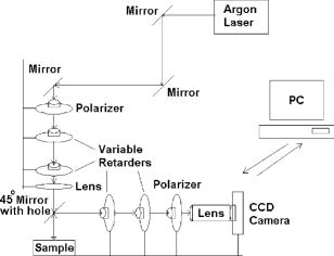
1.

Introduction

It is well known that through the characterization of the polarization effects in scattered light, useful information on the properties of turbid media can be obtained. As early as 1976, Bickel found that Bacillus Subtilis suspensions affected the angular distributions of the scattering matrix.¹ Expanding on this early work, Hielscher investigated how radial and azimuthal variations observed in diffusely backscattered polarization images of intralipid and polystyrene sphere suspensions changed with particle size, concentration, and the anisotropy factor.² Backman ³ and Bartlett ⁴ also demonstrated how polarized light scattering spectroscopy can be used to measure and characterize particle size distribution. In regards to in vivo tissue characterization, Demos ⁵ and Jacques ⁶ also reported on the use of backscattered polarized light for surface and subsurface imaging of biological materials. In these investigations, it was found that through the use of polarized light, the contrast of polarization-sensitive structures in tissue could be significantly enhanced to provide useful diagnostic information. Most recently, in 2004, Yaroslavsky ⁷ demonstrated how polarization-based reflectance and fluorescence imaging can be used for improved demarcation of skin tumors, and in 2005, Angelsky ⁸ investigated how the correlation structure of biological tissue polarization images can be used for cancer diagnostics. These investigations represent only a brief subset of the numerous and considerable advances in polarization-based biological measurements made over the past few years.

When describing photon migration in turbid media, common parameters of interest are the absorption coefficient, ${\mathrm{\mu }}_a$ , the scattering coefficient, ${\mathrm{\mu }}_s$ , and the scattering phase function. Although several methods may be used to experimentally measure these parameters, the inverse adding-doubling integrating sphere technique is a popular approach.⁹ Other useful optical parameters can also be experimentally measured by other approaches, such as by the method reported by Wang ¹⁰ In their investigation, a laser beam with an oblique angle of incidence was used to measure the reduced scattering coefficient of turbid media. Bevilacqua ^{11, 12, 13} also reported on local and superficial optical characterization of biological tissues achieved through spatially resolved diffuse reflectance at small source-detector separations. In these works, they investigated how extremely sensitive the determination of the absorption and reduced scattering coefficients are in relation to the phase function. However, regardless of the technique, most optical property measurement approaches only take into account the overall optical properties of the sample. In this paper, we present a technique to quantify the individual optical scattering coefficient contributions as a function of particle size for complex mixtures of polystyrene spheres. This technique exploits information encoded in the polarization-sensitive Mueller matrix, which is well known to provide a complete description of the polarization properties of an optical sample.^{14, 15, 16} In order to predict the scattering coefficient contribution for an individual particle size in complex suspensions consisting of a mixture of particle sizes, a partial least-squares (PLS) regression approach is employed. In addition, a stepwise chain selection algorithm, originally developed for wavelength selection in spectroscopy, was employed for spatial selection purposes.¹⁷ Through this spatial selection, an interpretation of the image-based Mueller matrices is provided, which sheds insight on the most relevant spatial positions and elements of the Mueller matrix. This step provides information on which elements of the Mueller matrix and the spatial information within the individual elements were used in the prediction of the particle-size-dependent scattering coefficient contributions.

2.

Theory

2.1.

Mueller Matrix/Stokes Vector Imaging

The polarization state for a given light field can be characterized by a Stokes vector, which is a $4\times 1$ vector:¹⁸

Eq. 1

$$S=\left[\begin{array}{c}\hfill I\hfill \\ \hfill Q\hfill \\ \hfill U\hfill \\ \hfill V\hfill \end{array}\right]=\left[\begin{array}{c}\hfill {⟨E_x{E}_x^{*}⟩}_{\tau }+{⟨E_y{E}_y^{*}⟩}_{\tau }\hfill \\ \hfill {⟨E_x{E}_x^{*}⟩}_{\tau }-{⟨E_y{E}_y^{*}⟩}_{\tau }\hfill \\ \hfill {⟨E_x{E}_y^{*}⟩}_{\tau }+{⟨E_y{E}_x^{*}⟩}_{\tau }\hfill \\ \hfill i({⟨E_x{E}_y^{*}⟩}_{\tau }-{⟨E_y{E}_x^{*}⟩}_{\tau })\hfill \end{array}\right]$$

where $E_x$ and $E_y$ are the electric field components parallel and perpendicular to a reference direction of light travel; $I$ is the total light intensity; $Q$ represents the tendency of the light to exhibit either horizontal or vertical linear polarization; $U$ represents the tendency of the light to exhibit either $+45°$ or $-45°$ linear polarization; and $V$ similarly represents the tendency of the light to exhibit either right or left circular polarization. The angle brackets, $⟨\dots {⟩}_{\tau }$ , represent the time average over the temporal integration time, which can be assumed to be much greater than the optical period. Due to the temporal integration, the time dependence of the electric fields is suppressed. A Mueller matrix is a $4\times 4$ matrix that describes how an incident Stokes vector, $S_{\mathrm{inc}}$ , is transformed by a given sample. In essence, the Mueller matrix can be thought of as an optical fingerprint of a sample. Therefore, if the Mueller matrix, $M$ , is known for a sample, the output or resulting Stokes vector, $S_{\mathrm{out}}$ , is given by

Eq. 2

$$S_{\mathrm{out}}=M{S}_{\mathrm{inc}}$$

If the Mueller matrix for a given sample is unknown, all 16 elements can be determined through the acquisition of 16, 36, or 49 intensity-based measurements corresponding to different combinations of input and output polarization states. ^{14, 15, 19, 24}

In our investigation, the polarization dependencies of the backscattered light from complex turbid media, consisting of mixtures of polystyrene spheres of different sizes, are investigated through image-based Mueller matrix polarization measurements. In these measurements, each element of an acquired Mueller matrix is a two-dimensional image rather than consisting of a single point. An example of an image-based Mueller matrix for a turbid phantom is shown in Fig. 1 , where the size of each element is $1.6\mathrm{cm}\times 1.6\mathrm{cm}$ and the image plane is taken at the surface of the sample. It should be noted that each element of the Mueller matrix corresponds to the same sample area; however, the observed differences represent different polarization dependencies as further described in Sec. 3.1.

Fig. 1

An experimentally measured Mueller matrix for a complex polystyrene mixture consisting of 0.2, 0.5, 1, and $2\mathrm{\mu }\mathrm{m}$ -diameter particles with respective scattering coefficient contributions of 0.5, 1.5, 0.25, and $5{\mathrm{cm}}^{-1}$ leading to an overall scattering coefficient of ${\mathrm{\mu }}_s=7.25{\mathrm{cm}}^{-1}$ .

3.

Materials and Methods

3.1.

Experimental Setup

The experimental setup, seen in Fig. 2 , is similar to that reported in our previous study.²⁵ An argon ion laser (Melles Griot, CA) is used as the light source, emitting at a wavelength of $514\mathrm{nm}$ with a power of $5.45\mathrm{mW}$ . The beam is initially polarized by a horizontal Glan Thompson polarizer (Melles Griot, CA). The input polarization state is controlled electro-optically with no moving parts via two liquid-crystal voltage-dependent variable retarders (Meadowlark Optics, CO) with the ability to alter the incident polarization state between horizontal (H), vertical (V), $+45°$ linear (P), and right circular (R). The polarized beam is then focused by a lens through a hole in a $45°$ mounted mirror onto the sample. The backscattered light from the sample is reflected through the output pathway consisting of two additional electro-optic variable retarders and a Glan–Thompson vertical polarizer. The output pathway is used to analyze the backscattered polarization state (e.g., H, V, P, R). The image is acquired by a thermoelectric-cooled $512\times 512$ 16-bit CCD camera (Apogee CCD, CA) fitted with a Nikon adjustable zoom lens. The sample Mueller matrix is calculated by 16 combinations of input and output polarization states. The Mueller matrix reconstruction is automated through a custom ${\mathrm{LabVIEW}}^{\circledR }$ program, which controls the CCD camera and the polarization states through a digital-to-analog (D/A) converter (National Instruments, Austin, TX).

Fig. 2

Experimental Mueller matrix backscattering imaging system.

4.

Results and Discussion

According to the methods described in Sec. 3, a PLS multivariate calibration model was formed from one set of Mueller matrix raw data consisting of a total of 60 phantoms, each representing a poly-disperse mixture of polystyrene spheres of different size spheres. Five latent variables were utilized in the calibration model, which was chosen based on the total possible number of different size spheres present in a single sample, four total, plus an additional one for the variation in water concentration. The use of five latent variables allowed the capture of high variance in both the transformed image intensities and the scattering coefficient contributions, 90.15% and 90.64%, respectively, while avoiding overfitting of the model to the data. Plots of predicted versus actual scattering coefficient contribution for every particle size within each of the 60 samples in calibration using the raw data set (i.e., unprocessed for spatial selection) are presented in Fig. 3 . The standard errors of calibration (SEC), summarized in the first column of Table 1 , for each particle size ranged from 0.3308 to $0.8582{\mathrm{cm}}^{-1}$ . In addition, to further validate the predictive capability of the computed model, a second set of independently collected data was used. In validation, the prediction results of scattering coefficient contribution for each particle size are shown in Fig. 4 and summarized in the second column in Table 1. Although the standard errors of prediction (SEP) as compared to SECs are larger in each case, in comparison to the overall range of scattering coefficient contributions being predicted, it does not appear that the calibration model is significantly overfitting the data. As can be partially seen in Fig. 3, although many data points overlap, the respective prediction errors for 0.2, 0.5, 1, and $2\mathrm{\mu }\mathrm{m}$ -diameter particles for zero concentration are 0.3144, 0.4238, 0.3381, and $0.3730{\mathrm{cm}}^{-1}$ , respectively. Based on this, the majority of the overall error contribution appears to be caused by prediction errors for the zero-contribution scattering coefficient (i.e., prediction error when a certain type of particle is not present in the sample). Therefore, signal and noise due to other particle sizes cannot completely be distinguished in the model.

Fig. 3

Scattering coefficient contribution prediction in calibration for (a) $0.2\mathrm{\mu }\mathrm{m}$ , (b) $0.5\mathrm{\mu }\mathrm{m}$ , (c) $1.0\mathrm{\mu }\mathrm{m}$ , and (d) $2.0\mathrm{\mu }\mathrm{m}$ -diameter spheres.

Fig. 4

Scattering coefficient contribution prediction in validation for (a) $0.2\mathrm{\mu }\mathrm{m}$ , (b) $0.5\mathrm{\mu }\mathrm{m}$ , (c) $1.0\mathrm{\mu }\mathrm{m}$ , and (d) $2.0\mathrm{\mu }\mathrm{m}$ -diameter spheres.

Table 1

Scattering Coefficient Contribution SEC and SEP for (a) Full Data Set and (b) Spatially Selected Data Set (SEC and SEP Units: cm−1 )

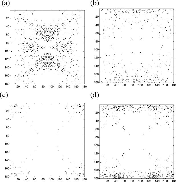
As an additional processing step, the raw data used in the previously described analysis were preprocessed before computing the calibration model with the PLS technique. The purpose of the preprocessing was to determine the most useful spatial locations in the overall Mueller matrix that provides accurate prediction of the scattering coefficient contribution for each respective particle size in the poly-disperse suspensions. To perform the spatial selection preprocessing, the method described in Secs. 2.3, 3.3 was employed. After preprocessing the raw data set, its overall size was reduced from 60 samples $\times \mathrm{121,500}$ , in length to 60 samples $\times \mathrm{2,999}$ , in length. Using the resampled data set, we formed a PLS multivariate calibration model. Again, five latent variables were utilized in the calibration model. For the spatially selected preprocessed data, the standard errors of calibration (SEC), summarized in the third column of Table 1, for each particle size ranged from 0.1585 to $0.7372{\mathrm{cm}}^{-1}$ and the overall errors were reduced in comparison to the unprocessed raw data in all cases, except for the $1\mathrm{\mu }\mathrm{m}$ -diameter spheres. In addition, to further validate the predictive capability of the computed model, the second set of independently collected data was resampled, choosing the same spatial locations used during calibration. In validation, the prediction results of scattering coefficient contribution for each particle size are summarized in fourth column of Table 1. As can be seen, similar standard errors of prediction (SEP) compared to the SEPs using the raw data set are observed; however, this was achieved using a considerably smaller subset of the original data size.

Although the use of spatial selection can considerably reduce the overall size of the data set needed for accurate prediction, it can also shed insight about the inherent structure of the data set and the location of relevant points useful in the prediction of the respective components (e.g., in this case, the scattering coefficient contribution for each respective particle size). In our experimental approach, the probing light has a wavelength of $514\mathrm{nm}$ , or $0.514\mathrm{\mu }\mathrm{m}$ . For particle sizes significantly smaller than the wavelength of light, scattering with properties as characterized by the Rayleigh approximation is more dominant; for particle sizes greater than the wavelength of light, scattering with properties as characterized by Mie theory is more dominant. Through the use of the employed spatial selection method, we can show that the type of scattering involved is directly encoded within specific areas of the Mueller matrix for each respective particle size. To illustrate this, the Mueller element $M_{12}$ was chosen (see Fig. 5 ). In the $M_{12}$ element, it can be seen for the $0.2\mathrm{\mu }\mathrm{m}$ particle size, Fig. 5a, where Rayleigh scattering was dominant, considerable locations near the center of the element were used in prediction. In addition, locations to represent or preserve the azimuthal variations in the element were also selected. As the particle size begins to approach the wavelength of light (e.g., for the $0.5\mathrm{\mu }\mathrm{m}$ particle size), as shown in Fig. 5b, several locations throughout the $M_{12}$ element were chosen, although there is less information chosen to preserve the azimuthal variations. For particles sizes greater than the wavelength of light (e.g., for the $1\mathrm{\mu }\mathrm{m}$ and $2\mathrm{\mu }\mathrm{m}$ particle sizes) where Mie scattering dominates, less information was chosen near the center of the element and more information along the $+45°$ and $135°$ angles increasing toward the outer boundary of the element was chosen. Therefore, this is indicative of how the scattering type is encoded within the Mueller matrix. Similarly, results were seen to a lesser degree for other specific elements in the Mueller matrix as well. Other information, such as particle shape, would be expected to be encoded in the Mueller matrix in a similar fashion and will be the focus of future investigations.

Fig. 5

Spatial selection results for the $M_{12}$ element. Dots indicate points in the $M_{12}$ element that were chosen to predict the scattering coefficient contribution for (a) $0.2\mathrm{\mu }\mathrm{m}$ , (b) $0.5\mathrm{\mu }\mathrm{m}$ , (c) $1.0\mathrm{\mu }\mathrm{m}$ , and (d) $2.0\mathrm{\mu }\mathrm{m}$ -diameter spheres.

5.

Conclusion

By the use of backscattered polarized light imaging in turbid media, we have shown, in part, how variations in image-based Mueller matrices encode information on the scattering type, particle size, and particle concentration. Furthermore, methods such as the PLS technique can be employed in the formation of mathematical models to quantitatively predict scattering coefficient contributions as a function of particle size. In future investigations, further extensions to improve the robustness of such modeling approaches to handle increasingly complex media such as those with non-uniform spatial distributions and differing particle geometries may eventually allow such methods to be potentially used as a diagnostic tool to distinguish between tissue types and abnormalities that have differences in cellular structures and tissue components.