2.1.

Preparation and Sound Stimulation

Adult guinea pigs of both genders weighing between $250\text{to}500\mathrm{g}$ were used in accordance with the rules approved by the local ethics committee (permit N311/03). Detailed descriptions of the preparation have been published previously.^{7, 8} Only a brief description is given here. The excised temporal bone was sealed to a holder and immersed in tissue culture medium [minimum essential medium (MEM) with Earle’s salts, Gibco, Palsley, UK]. The external auditory canal was attached in the holder to face a loudspeaker, thus enabling sound stimulation. To gain access for imaging as well as to establish a perfusion system, a portion of the bony shell covering the apical part of the cochlea was carefully removed. A perilymph-like oxygenated solution (MEM) was used to perfuse scala media via an opening in the basal turn of the cochlea. The fluorescent dye calcein acetoxymethyl ester (Molecular Probes, Leiden, the Netherlands, $4\text{-}\mu \mathrm{g}∕\mathrm{ml}$ concentration) was also delivered by perfusion system to stain Reissner’s membrane and the supporting cells of the organ of Corti. The medium was then exchanged and $12.5\mu \mathrm{g}∕\mathrm{ml}$ of the dye RH 795 was added to the perfusion system. This styryl, potentiometric dye labels preferentially cell membranes of the sensory cells and nerve fibers. The overall condition of the preparation was routinely assessed using a low magnification lens. In the case of structural damage, swollen sensory cells, or other abnormalities, the preparation was discarded. For imaging we used a Carl Zeiss LSM510 laser scanning confocal microscope equipped with a $40\times$ , NA 0.8 water immersion lens. Pixel sizes were in the range $50\text{to}100\mathrm{nm}$ . Due to anatomical constraints, a perfect profile view of the organ of Corti cannot be acquired. However, if the preparation is rotated with respect to the optical axis of the microscope, images that are quite close to true cross sections can be obtained. In this study, sound stimulation was applied in a range of frequencies between 100 and $600\mathrm{Hz}$ . The frequencies, at which the imaged section responded most, ranged between 150 and $225\mathrm{Hz}$ . Stimulus levels were between 88 and $110\mathrm{dB}$ sound pressure level (SPL). Due to the immersion of the preparation, the middle ear is fluid filled, which, along with the opening of the apical turn, reduces the effective stimulus level by $20\text{to}30\mathrm{dB}$ .⁹ The data presented in this text were not corrected for this attenuation.

2.2.

Image Sampling and Noise-Free Phase Extraction

A schematic overview of the acquisition system is shown in Fig. 1 . Note that the LSM controller outputs a timing signal for each pixel acquired. This pixel clock is used as the time base for the stimulus generation by an A/D board (PCI-6115, National Instruments, Austin, Texas). Thus, when a new pixel is acquired by the LSM, a new sample of the stimulus is written to the output of the A/D board. In the previous version,⁶ the sound was generated by a function generator and sampled. The phase of the sound was estimated and pixels sorted to have approximately the same temporal relation to the stimulus. With this old method, noise in the sound channel influenced the recorded phase, and therefore the reconstructed images did not have an absolutely fixed temporal relation to the stimulus. These problems yielded artifacts, which limited the resolution of the technique. In the present setup, the discrete-time stimulus is generated by software (LabView 7.1, National Instruments, Austin, Texas), and the phase argument of each sound sample (one sample corresponds to one pixel) is saved and used for Fourier series extraction. This new image sampling technique and the noise-free phase extraction yield less artifacts in the reconstructed images due to low-pass filtering of the time series and an absolutely fixed temporal relation between images and stimulus.

Fig. 1

Schematic overview of the acquisition system. The basic principle is to use the pixel clock of the LSM as a time base for the generation of the sound stimulus. This ensures synchronization between image acquisition and stimulus generation. The phase of the sound stimulus for each pixel is then saved for processing.

2.3.

Fourier Series Extraction

During experiments, a fixed number of images $\left(N_1\right)$ are acquired without an interframe delay. At the same time, the phase array of the stimulus is saved with dimensions equal to the image stack. Because the pixel value $\left(I_m\right)$ and the phase $\left(P_m\right)$ of each pixel are known, a Fourier series may be used to reconstruct an image sequence where all pixels in a given frame have an identical temporal relation to the sound stimulus. To illustrate this, imagine a sample of a tiny bright structure surrounded by darker ones, which results in one bright pixel in the image. If the sample moves periodically in the image plane, the intensity will drift out of the bright pixel into a darker one and back again, according to the motion direction. Plotting the intensity of the bright pixel as a function of the motion phase will yield a periodic behavior, which can be analyzed by a Fourier series approach.

The Fourier series coefficients are computed for each pixel location along the time dimension, which maps to the phase domain.

2.4.

Optical Flow Calculations

A wavelet-based differential optical flow algorithm was used to quantify the motion seen in the image sequences. A detailed description of this algorithm and a thorough performance characterization can be found in Ref. 10. In general, direct comparisons show that the performance of this optical flow algorithm is similar to the standard Lucas-Kanade method¹¹ when noise-free image sequences are used. Under more realistic conditions, where noise is added to the image sequence, the wavelet-based algorithm has a higher density of correct motion estimates.

2.5.

Calibration Experiments

To test the acquisition system described, rigid autofluorescent samples were attached to a vibrating piezoelectric translator (P841.10, Physik Instrumente, Karlsruhe, Germany). The motion amplitude of the piezoelectric translator was measured by a built-in strain gauge sensor, which was calibrated by an interferometer. Due to mechanical limitations of the microscope setup, the translator had to be attached to one end of a $10\text{-}\mathrm{cm}$ -long rod, which was mounted at the opposite end. The sample itself was glued to the head of a $2\text{-}\mathrm{cm}$ -long screw, and the screw was mounted in the piezo head. The calibration experiments are influenced by the mechanical mount, which could not be used during the interferometric measurements. This may influence the magnitude and frequency responses, especially in the direction perpendicular to the one of the applied motion. By aligning the piezoelectric translator to one axis of the image, it is possible to separate the parallel and the perpendicular component of the motion relative to the translator elongation axis.

The samples were imaged with the same objective lens used during real experiments. However, it is not possible to use water immersion during these calibration experiments; the effective numerical aperture of the lens is therefore decreased and the image quality worse than that found during real experiments. In this regard, the calibration experiments described next represent worst-case estimates.

3.1.

Artificial Target Tests

Figure 2 (A) shows an image of a test sample, consisting of a piece of autofluorescent plastic attached to the piezo stack. Note that the scale of the structural details of the target matches approximately the one typically found in biological samples. In the first set of experiments, the piezoelectric translator was vibrating at $200\mathrm{Hz}$ . Figure 2(B) shows the relative motion amplitudes parallel to the piezo-elongation direction. A systematic overestimation of motion amplitudes occurs when displacements in the order of the pixel size $\left(112\mathrm{nm}\right)$ or larger are to be measured. Compared to the physical motion, the measured motion is about 25% too large for motion amplitudes close to the pixel size and drops to 14% for motion amplitudes of roughly eight times the pixel size. This behavior is relatively independent of the number of images in the acquisition. This is not so surprising, since the signal-to-noise ratio in the images is very good (pixel time $6.4\mu \mathrm{s}$ ). We also tried to use just four frames in the acquisition, which failed in most of the cases, because the noise influence increases dramatically when fewer frames are acquired. The dependency of the errors on the number of acquired frames becomes more serious at a faster scan speed (pixel time $2.5\mu \mathrm{s}$ ), because the signal-to-noise ratio is much worse. Therefore scanning faster to reduce the laser exposure time of the biological sample is yielding larger errors. To get the same errors with faster scan speeds, one needs to scan more frames. Hence the laser exposure time is almost the same as with slower scan speeds.

Fig. 2

(A) Micrograph showing an autofluorescent piece of plastic used for initial calibration (pixel size $112\mathrm{nm}$ ). (B) Motion measured from the reconstructed image stack by the optical flow algorithm is compared to the real, physical motion of the piezoelectric translator. Physical motion was measured with a built-in strain gauge sensor. (C) Relative standard deviation of the estimated motion distribution as a function of the applied motion. (D) Angular errors as a function of the applied motion.

The accuracy depends to some extent on the number of harmonics included in the reconstruction. Although similar values are obtained for small displacements, results are improved at large displacements if two harmonics are used in the reconstruction. Adding more harmonics than two did not appreciably alter the accuracy (data not shown). The width of the motion estimate distribution for one acquisition is described by the standard deviation relative to the applied motion [see Fig. 2(C)]. In essence, this number describes the variability inherent to one motion trajectory. It is smaller than 10% when motions larger than the pixel size are applied. The situation changes when motions smaller than the pixel size are applied. Figure 2(B) shows an overestimation of this motion of roughly 25 to 30%; note that this part of the graph is very noisy. The reason for this can be seen in Fig. 2(C), where the relative standard deviation increases drastically (up to 40%) for motions smaller than the pixel size.

The motion estimate is limited by the noise in the acquired images, giving rise to a virtual motion. To access these limitations, we acquired a time series of images when the sample was not moving. The estimated motion amplitudes of these acquisitions was always smaller than $10\mathrm{nm}$ , with standard deviation of less than $6\mathrm{nm}$ (pixel size $112\mathrm{nm}$ ) and $5\mathrm{nm}$ with standard deviation of less than $3\mathrm{nm}$ (pixel size $56\mathrm{nm}$ ). This is comparable to the one measured in a real temporal bone experiment, where the estimation of the virtual motion is below $10\mathrm{nm}$ .

By measuring the angle of the major axis of the motion trajectories, it is possible to assess the angular error of the motion estimate. For motions larger than the pixel size, the angular error is below $2\mathrm{deg}$ . It increases for motions smaller than the pixel size, but remains smaller than $10\mathrm{deg}$ . The angular error is not substantially affected by the amount of acquired frames. The error of the motion estimation depends to some extent on the structure of the sample, especially on the characteristic length scale over which contrast occurs. If this length scale is smaller than the pixel size, the pixel size is the limiting factor.

Figure 3 (A) shows the same target at higher zoom (pixel size $56\mathrm{nm}$ ). The translator was vibrating at $200\mathrm{Hz}$ . We applied motion on the order of the pixel size and smaller. Figure 3(B) shows the relative motion amplitudes. The motion is overestimated by 20 to 30%. The relative standard deviation of the estimation, shown in Fig. 3(C), is again very small for motions on the order of the pixel size, and increases dramatically as the applied motion becomes smaller. Figure 3(C) also shows that the amount of acquired frames has an influence on the width of the estimate distribution. For displacements larger than half the pixel size, there is almost no difference between 8, 12, and 20 frames scanned. But at motions much smaller than half the pixel size, the width of the estimate distribution for 20 frames scanned is only $2∕3$ of the one with 8 or 12 frames scanned. This means that at these small displacements, the noise in the image acquisition limits the information content of the motion in the images. Therefore it is necessary to scan more frames to reduce the uncertainty in the motion estimation. The frequency dependence of the motion estimation [Fig. 3(D)] shows a resonance-like behavior, with a broad maximum around $300\mathrm{Hz}$ and a dropoff to each side. This behavior has been observed with all test samples and also at different scan speeds (data not shown). Therefore it may reflect the mechanical properties of the sample mount (see calibration experiments in Sec. 2.5).

Fig. 3

(A) Calibration sample at higher zoom than Fig. 2 (pixel size $56\mathrm{nm}$ ). (B) The mean motion estimate relative to the physical applied motion. (C) Standard deviation of the estimated motion distribution relative to the applied motion. (D) Relative motion estimated as a function of the applied frequency.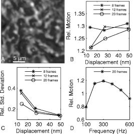

Thus it is concluded that this acquisition system performs very well. Optimum performance is achieved for motions about the size of a pixel, and it would therefore make sense to adjust the pixel size of the microscope according to the expected size of the motion. Two harmonics should be included in the calculations. The number of acquired frames has a relatively small influence. Note that these minor estimation errors are not caused by the optical flow algorithm, but rather by the acquisition system itself. When using image sequences with computer-generated translations, motion was accurately measured, even for very small displacements and even if the image sequence was substantially degraded by noise (data not shown).

3.2.

Cochlear Motion Data

We have also obtained vibration data in several temporal bone preparations. An example is shown in Fig. 4 (A). The image of these two outer hair cells was obtained in situ during simultaneous sound stimulation at the characteristic frequency $225\mathrm{Hz}$ , at a stimulus level of $97\text{-}\mathrm{dB}$ SPL (the effective stimulus level is reduced by immersion of the preparation and by the opening of the apical turn). The asterisk in the image marks a point on the reticular lamina, the motion of which is shown in Figs. 4(B)-(D). The three motion trajectories display the motion for three different frequencies (at the characteristic frequency, below, and above it). Changing the stimulus frequency altered the overall displacement amplitude, but the shape and orientation of the trajectories remained similar across frequencies. The main axis of the trajectories approximately coincided with the long axis of the outer hair cells. This vibration component dominated the response; components in other directions were generally quite small.

Fig. 4

(A) Two outer hair cells from the second and third row. The image was obtained during sound stimulation at $225\mathrm{Hz}$ . (B), (C), and (D) Motion trajectories at the characteristic frequency, at 150 and at $400\mathrm{Hz}$ , respectively.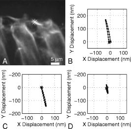

In Fig. 5 , a tuning curve obtained from this preparation is plotted. For comparison, we also include a previously published tuning curve, which was measured with a laser interferometer.⁷ The overall shape of the curves is similar, as are the response amplitudes. In both cases, a notch is seen on the high-frequency side of the curve, although the notch appears more pronounced in the recently measured dataset. Although both curves were obtained in isolated preparations, they are quite similar to those seen in living, anesthetized animals.¹²

Fig. 5

A tuning curve measured from the same preparation as in Fig. 4 is plotted together with a displacement tuning curve measured at $93\mathrm{dB}$ SPL (Ref. 7).