1.

Introduction

Light has been used to probe multiple scattering media such as tissue (or tissue-mimicking phantoms) to map both their mechanical^{1, 2} and optical properties.³ Photon-propagation-based optical property recovery has now grown to a discipline on its own merit, diffuse optical tomography (DOT), which has proven applications in diagnostic imaging based on absorption coefficient variations associated to pathology.^{4, 5, 6} The visco-elastic properties are also obtained from light scattering measurements through estimation of mean-square displacements of an ensemble of embedded tracer particles, subjected to intrinsic thermal stress.⁷ External loading of scattering centers is also in vogue by such means as the application of magnetic field on magnetic tracer particles^{8, 9} and laser tweezers.¹⁰ Under this category, turbid media are also subjected to modulation by ultrasound (US) pressure, applied by either parallel or focused ultrasound beams and interrogated by a coherent light beam. Light scattering studies in turbid media modulated by ultrasound have shown that the presence of US-tagged photons in the transmitted light results in the modulation of the detected intensity (or amplitude) autocorrelation.¹¹ The depth of modulation is influenced by the local absorption coefficient of the medium insonified by the US beam. This result added an extra dimension to DOT imaging, allowing the possibility of spatial resolution improvement of absorption coefficient images by discarding all detected diffuse photons except those tagged by ultrasound. The flurry of activity in this direction saw the arrival of a new branch of DOT known as ultrasound-assisted optical tomography (UAOT).^{12, 13, 14}

However, it was only recently that the influence of the local microrheological properties of the turbid medium on the UAOT measurement (which is the depth of modulation of the intensity or amplitude autocorrelation) has been investigated. Since the US beam subjects the scattering centers in the object to an extra periodic stress, in addition to the thermal stress, the modulation in the detected photon correlation is also related to the amplitude of vibration of the scattering centers. This amplitude, in turn, is influenced by the local visco-elastic properties.¹⁵ In Ref. 15 it is shown that the depth of modulation in the autocorrelation is influenced by the amplitude of vibration $u$ of the scattering centers and $\mathrm{\Delta }n$ the modulation of the refractive index because of insonification, in addition to the local absorption coefficient. In fact, the phase modulation suffered by light owing to $\mathrm{\Delta }n$ and $u$ results in modulation of the detected intensity, providing a carrier whose amplitude is influenced by the local absorption coefficient in the region of insonification through multiplication.

In Ref. 15 it is pointed out that if the UAOT read-out is to be employed for a quantitatively accurate recovery of either the optical or elastic properties of the object, the influence each of these has on the modulation depth has to be first estimated and accounted for. Out of these, the contribution of absorption can be independently estimated, by reconstructing the absorption coefficient distribution using the established DOT reconstruction algorithm on the measured intensity autocorrelation $g_2\left(\tau \right)$ at $\tau =0$ , which is the same as the intensity data. The remaining contributions are from refractive index fluctuations $\left(\mathrm{\Delta }n\right)$ and the path length fluctuations $\left(u\right)$ . We show in this work that the displacement introduced by the focused US beam in the region of insonification is along the axis of the US transducer. Therefore, assuming that tissue-like material has a scattering anisotropy $g$ of $\sim 0.9$ (light scattering is forward directed), the path length modulation and its variation with elastic property picked up by light launched perpendicular to the US transducer axis is small compared to that picked up by light along the transducer axis. This variation is negligible for storage modulus above $\sim 50\mathrm{kPa}$ , which is slightly above the normal value of healthy breast tissue.¹⁶ In addition, it is shown through simulations and experiments that the modulation in $g_2\left(\tau \right)$ for light launched along and perpendicular to the US axis approach the same constant pedestal value as the storage modulus of the material is increased beyond $80\mathrm{kPa}$ . [This value of storage modulus is dependent also on the power input through the US transducer. When the radiation force from the US force increases, significant displacement components still influence the $g_2\left(\tau \right)$ modulation depth, much beyond the $80\text{-}\mathrm{kPa}$ limit of the present experiments.] This implies that for such large stiffness, the displacement of tissue particles introduced by US radiation force is negligibly small, and the contribution to modulation in $g_2\left(\tau \right)$ is entirely because of $\sum \mathrm{\Delta }{n}_j{\ell }_j$ , where ${\ell }_j$ is the average undisturbed scattering path length in the insonified region. This pedestal value to which the $g_2\left(\tau \right)$ modulation approaches is the same for both axial and transverse light interrogation, in spite of the fact that the length of interaction for these two cases is not the same. The axial length of the US focal region is approximately four times its width at the center (see Sec. 2). But the path length modulation that can be picked up in diffusing wave spectroscopy has a maximum value of $\lambda$ , the wavelength of the interrogating light.¹⁷ For this reason the $g_2\left(\tau \right)$ modulation depth in the two directions of interrogations approaches the same value when the storage modulus is large. This residual value, which is insensitive to storage modulus variations for storage modulus beyond $50\mathrm{kPa}$ for transverse illumination and $80\mathrm{kPa}$ for axial illumination, is the contribution from $\mathrm{\Delta }n$ . This means that for other values of storage modulus, wherein the $g_2\left(\tau \right)$ modulation has contribution from both displacement and $\mathrm{\Delta }n$ , the contribution from $\mathrm{\Delta }n$ can be subtracted out, and the modulation arising entirely out of displacement of scattering centers can be ascertained. This paves the way for retrieving the displacement components induced by the US force from measurement of $g_2\left(\tau \right)$ modulation depth, which can be used for quantitative reconstruction of the storage modulus.

As a consequence of the previous observation, we suggest through this study that the absorption coefficient map obtained from $g_2\left(\tau \right)$ modulation depth in an UAOT experiment is least likely to be affected by storage modulus variations (which certainly accompanies malignant regions along with absorption coefficient increase) when the interrogation light is perpendicular to the US transducer axis and the insonification is from a focused US transducer. In this case, the contribution to $g_2\left(\tau \right)$ modulation depth from displacement is significantly less and varies very little with storage modulus. The summary of the work reported here is as follows. In Sec. 2 the force distribution in the focal region of the US transducer is calculated by solving the Westervelt equation¹⁸ for the input parameters of the transducer and the acoustic properties of the phantom used in the experiments later. The force distribution is used in the forward elastography equation in Sec. 3, which is solved for the tissue-mimicking phantom, assuming it to be purely elastic. It is seen that the estimated displacement distribution is along the US transducer axis. Section 4 describes the simulation of propagation of photons through the insonified phantom. The goal of the simulation is the estimation of $g_2\left(\tau \right)$ and its modulation. Photons are transported both along and perpendicular to the axis of the US transducer. Section 5 reports the experimental verification of the simulations on special tissue-mimicking phantoms. In this section, the results of simulation are compared with the corresponding experimental results. In Sec. 6 the results are discussed, and Sec. 7 puts forth the concluding remarks.

2.

Force Distribution in the Focal Region of the Ultrasound Transducer

The object, which is a slab of tissue-mimicking material, is insonified by radiation from a focusing US transducer. The tissue particles in the focal region are set in vibratory motion by the force of the US beam. In this section, our objective is to find the force distribution in the focal region of the transducer. This can be obtained from the oscillatory force experienced by the tissue particles, which is given by

In this work, Eq. 3 is solved numerically for $p$ in the focal region of a focusing ultrasound transducer using the procedure described by Kamakura, Ishiwata, and Matsuda.¹⁸ For this, the Westervelt equation is first written in an oblate spheroidal coordinate system, which helps one to write it as two separate spheroidal beam equations: one valid in the focal region of the transducer, where the nonlinearities have to be invoked and the wave is assumed plane; and the other close to the source, where the wave is assumed to be spherically converging. The pressure waves, which are distorted owing to the presence of the nonlinear terms, are expanded using the Fourier series, which results in two sets of coupled nonlinear partial differential equations (PDEs) (the two sets are for the two regions) for the Fourier coefficients. These PDEs are solved numerically using the finite difference scheme.¹⁸

The details of the US transducer used in the experiments, and borrowed herein for the simulations, are as follows. The central frequency of operation $\omega =1\mathrm{MHz}$ , focal length of the transducer $\left(d\right)$ is $50\mathrm{mm}$ , and its aperture radius $\left(a\right)$ is $25\mathrm{mm}$ , giving a full aperture angle of $60\mathrm{deg}$ . The tissue properties are taken to be those of the tissue-mimicking phantoms used in our experiments: average sound $\mathrm{velocity}=1545{\mathrm{msec}}^{-1}$ , sound absorption $\mathrm{coefficient}=1\mathrm{dB}∕\mathrm{cm}$ at $1\mathrm{MHz}$ , and density $\rho =1000\mathrm{kg}∕{\mathrm{m}}^3$ . The US transducer is of continuous wave type and is assumed to operate at a constant frequency. The electrical input to the transducer is adjusted such that the pressure at the transducer surface is $7.5\mathrm{kPa}$ .

We have used the procedure of Ref. 18 to estimate the pressure at the focal region. The focal region itself is seen to be ellipsoid in shape with a large eccentricity. The axial extent of the focal region is seen to be four times its width at the center. The cross sections (the radial and axial) through the center point of the ellipsoidal region of the estimated pressure distribution are shown in Figs. 1a and 1b .

Fig. 1

(a) The cross sectional plot of the normalized pressure distribution $\overline{p}=p∕p_0$ in the focal region of the transducer, where $p_0$ is the pressure at the transducer surface $\left(7.5\mathrm{kPa}\right)$ . The plot is along the axial direction (i.e., $z$ direction) through the center of the ellipsoidal focal region. The axial distance is normalized as $(z∕d)$ , where $d$ is the focal length of the transducer. (b) The plot is along the radial direction at the plane $z=0$ . The radial distance is normalized as $r∕a$ , where $r$ is the radial distance and $a$ is the transducer aperture radius.

Using the estimated pressure distribution from Eq. 3, the intensity in the focal region is estimated.²⁰ For the specifications of input voltage for the transducer, the calculated maximum intensity is found to be within the safety limits stipulated by the Food and Drug Administration (FDA).²⁰ The pressure distribution is used to arrive at the force exerted by the US wave in the focal region, which is employed in Sec. 3 in the elastography equations to estimate the resulting displacement distribution in the focal region.

3.

Computation of the Displacement Field in the Focal Region of the Ultrasound Transducer

In the previous section we have calculated the distribution of force vector in the focal region of the US transducer. The force in the focal region is sinusoidal and is along the transducer axis. In this section we use the equilibrium equations of elasticity to estimate the amplitude of vibration of tissue particles set in motion by the applied force. For rendering the computation tractable, the following assumptions are made: 1. the region of insonification is assumed to be a rectangular slab inscribed inside the estimated ellipsoidal focal region, and 2. the force distribution is assumed constant in all the voxels in the slab and kept equal to the average force in the ellipsoidal region.

The governing equation for the tissue displacement $u=(u_1,u_2,u_3)$ loaded by a vibrating force $F_0\cos \omega t$ along the transducer axis [the transducer axis is taken along the $z$ axis: Fig 2 ] is given by²¹

Fig. 2

The schematic diagram of the experimental setup. A continuous-wave, concave US transducer ( $1\mathrm{MHz}$ , with a hole at the center of the aperture) is used to insonify the phantom. The insonified focal region is interrogated by an unexpanded laser beam ( $\mathrm{He}\text{-}\mathrm{Ne}$ , $632.8\mathrm{nm}$ ), which passes coaxially along the transducer axis in (a). The light exiting is collected using a single-mode fiber to a photon counting PMT (single unit consists of a PMT and pulse amplifier discriminator) and a correlator. (b) Here the light interrogates the focal region perpendicular to the axis of the US transducer.

A typical solution of $u=(u_1,u_2,u_3)$ for the specifications of the transducer used in the experiments and representative values of $E^e$ $\left(11.39\mathrm{kPa}\right)$ , $\nu$ (0.499), and $\rho$ $(1000\mathrm{kg}∕{\mathrm{m}}^{3)}$ for the phantom is given by $u_1=4.28\times {10}^{-18}\mathrm{mm}$ , $u_2=2.57\times {10}^{-17}\mathrm{mm}$ , and $u_3=72.87\times {10}^{-6}\mathrm{mm}$ .

We underline that the displacement vector is almost along the transducer axis (here in the $z$ direction). This pattern is repeated when the object parameters are varied to represent a spectrum of mechanical stiffness. The prior computation is repeated also for a larger object of dimensions $50\times 45\times 15\mathrm{mm}$ , which also confirmed our observation that the displacement is along the transducer axis.

In the next section, we describe the interaction of photon packets launched, both along the transducer axis and perpendicular to it, with the focal region in the object where the scattering particles are set in motion by the applied force.

4.

Interrogation of the Insonified Object with Light

As seen in the last section, we have set the particles of the object at the focal region of the US transducer into vibratory motion through the force applied by the US pressure, which also produces periodic compression and decompression resulting in the modulation of refractive index. In this section we interrogate the focal region of the US transducer with a coherent light beam, so that the phase modulation picked up by the light can be read out from measurements made at the boundary. The measurement on the exiting photons is the intensity autocorrelation $g_2\left(\tau \right)$ of photons detected through a photon-counting detector. It is well known^{12, 13} that the presence of the ultrasound-tagged photons manifests itself as modulation on $g_2\left(\tau \right)$ , whose depth is affected by the optical absorption coefficient of the insonified region and the optical path length modulation effected by the US beam. We assume that the set of objects used in our simulations to study the effect of storage modulus variations on $g_2\left(\tau \right)$ has constant and homogeneous absorption coefficient distribution (which is also ensured in the experiments). That leaves us only with the optical path length modulation. The optical path the photons take during the $j$ ’th scattering event is $l_{j}n$ in the absence of US insonification, which becomes $(l_j+u_0)(n+\mathrm{\Delta }n)$ with the insonification. Here, $u_0$ is the component of displacement of the $j$ ’th scatterer in the direction of $l_j$ , and $\mathrm{\Delta }n$ is the local modulation in $n$ , owing to the US beam. Therefore, assuming $u_0$ and $\mathrm{\Delta }n$ to be small and neglecting the term containing the product $u_0\mathrm{\Delta }n$ , the optical path length modulation to light at the $j$ ’th scattering event is given by

Details of computation of $F\left(\tau \right)$ are given in Ref. 22, as are expressions for $\mathrm{\Delta }{\varphi }_{n,j}(t,\tau )$ and $\mathrm{\Delta }{\varphi }_{d,j}(t,\tau )$ . These are

Launching and tracking a large number of photons through Monte-Carlo (MC) simulations can also estimate the field autocorrelation. The MC simulation is computation intensive, and to reduce the computational burden, the following suggestions from Ref. 22 are incorporated in the procedure and implemented here. 1. The point detector is replaced by a large area plane detector, justified by the reciprocity principle of light diffusion. 2. The object is assumed to have an isotropic scattering coefficient of ${\mu }_s^{\prime }=(1-g){\mu }_s$ , which means that ${\ell }^{*}$ , the transport mean-free path length, is the basic step length used in MC simulations (and not the scattering mean-free path length). The similarity relation valid for light diffusion in highly scattering media justifies the second assumption. The perturbation in the path length is estimated by solving the forward elastography equation for the focal region. (The US transducer input power is adjusted so that the force in regions outside the focal volume is small and hence also the resulting displacements.) We estimate the perturbation in refractive index $\mathrm{\Delta }{n}_j$ using $(\partial n∕\partial p)$ value for soft tissue and the pressure estimated in Sec. 2.

To evaluate $g_1\left(\tau \right)$ , we compute through MC simulations both the detected photon weights and the optical path traversed by the photon through the object. From $g_1\left(\tau \right)$ , $g_2\left(\tau \right)$ is estimated, again using the Siegert relation. The strength of the power spectrum is estimated by finding the area under the peak at $1\mathrm{MHz}$ of the Fourier transform of $g_2\left(\tau \right)$ . The power spectral component is proportional to the depth of modulation in $g_2\left(\tau \right)$ . Simulations are carried out launching photons along the US transducer axis and perpendicular to it (Fig. 2), so as to intercept the focal region.

The simulation results, which are discussed in Sec. 6, always showed a larger modulation depth in $g_2\left(\tau \right)$ for light traversed along the axis than perpendicular to it. The reasons for this are as follows. 1. The component of amplitude of vibration (which is along the transducer axis) picked up by the axially launched photons are much larger compared to that picked up by the photons launched in the transverse direction. The result is that the phase modulation in the axial photons is contributed by $\mathrm{\Delta }n$ and a larger component of the vibration amplitude $u$ . For the transverse photons, the contribution from $u$ is smaller. 2. Photons launched along the axis had a four times larger length of interaction with the insonification region than those launched perpendicular to the axis. We show through both simulations and experiments that when the storage modulus of the object is increased, the modulation depth in $g_2\left(\tau \right)$ measured from axial photons decreased rapidly, whereas the same measurements from the transverse photons showed smaller absolute modulation depth and range of variation (see Fig. 3 ). As indicated in the Introduction and demonstrated in Fig. 3, when the storage modulus increased, the modulation depth in $g_2\left(\tau \right)$ measured from transverse and axial light approached the same constant value. Since with increase in storage modulus the amplitude of vibration decreased, this fall-off of the detected modulation depth indicated the decreasing contribution of vibration amplitude of particles to the overall modulation of light. These results are further discussed in Sec. 6.

Fig. 3

Plots showing the variations of the measured power spectral amplitude at $1\mathrm{MHz}$ with respect to the storage modulus $\left(G^{\prime }\right)$ of the phantom. The absorption coefficient of the phantom is kept constant at $2.5\times {10}^{-4}{\mathrm{mm}}^{-1}$ . The curve A is for measurement done for photons interrogating the focal region axially, and curve B is the same for photons launched in the transverse direction. Solid lines represent results from simulations (or theory) and the symbols are from the experimental measurement. The power spectral amplitudes measured in the transverse directions are not significantly affected by changes in the elastic property of the phantom compared to axial measurements.

In our theoretical simulations, we have used both the analytical expression arrived at on the basis of Eq. 12 ²² and the MC simulation to estimate $g_1\left(\tau \right)$ , and through it $g_2\left(\tau \right)$ , and the power spectral component at the US frequency. The typical values for tissue optical properties used in the simulation are absorption $\mathrm{coefficient}=2.5\times {10}^{-4}{\mathrm{mm}}^{-1}$ , $4.4\times {10}^{-2}{\mathrm{mm}}^{-1}$ , and $6\times {10}^{-2}{\mathrm{mm}}^{-1}$ , scattering coefficient=1.441 to $4.5{\mathrm{mm}}^{-1}$ , anisotropy factor=0.9, and refractive index=1.34. The values of storage modulus are 11.4, 23.4, 43.7, 51.2, and $97.3\mathrm{kPa}$ . The average sound velocity in tissue is assumed to be $1545\mathrm{m}∕\sec$ . The simulations are repeated for photons launched along and perpendicular to the transducer directions.

The results showing variation of modulation depth with optical and mechanical properties are shown in Fig. 4 , which are further discussed in Sec. 6. We would like to mention that the modulation depths obtained through the theoretical expression for $g_1\left(\tau \right)$ and MC simulation agreed with one another very well. Therefore, in Figs. 4a, 4b, 5 , the simulation results can be taken as those obtained through either of these means.

Fig. 4

(a) Plots showing the variation of the power spectral amplitude at $1\mathrm{MHz}$ with respect to the storage modulus $\left(G^{\prime }\right)$ of the phantom (size $10\times 10\times 10\mathrm{mm}$ ). The power spectral amplitudes are normalized with respect to the maximum value available in the set. The photons are launched along the axis of the US transducer. Curves A, B, and C are obtained for ${\mu }_a=2.5\times {10}^{-4}$ , $4.4\times {10}^{-2}$ , and $6\times {10}^{-2}{\mathrm{mm}}^{-1}$ , respectively. Solid lines represent results from MC simulations and the symbols are from experimental measurement. For the axial launch of photons, as the storage modulus increases the range of variation in the measured power spectral amplitude has become smaller for the same range of ${\mu }_a$ variation. (b) These are the same as in (a) but for a phantom of dimensions $50\times 40\times 15\mathrm{mm}$ . The type of variation of power spectral amplitude with ${\mu }_a$ and storage modulus is the same as in (a).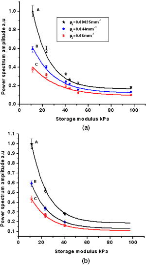

Fig. 5

The plots showing the variation of power spectral amplitude with scattering coefficient of the phantom. The light is launched along the axis of the transducer and the dimension is $10\times 10\times 10\mathrm{mm}$ . Curve A compares experimental measurements from the phantom with MC simulation results, where the scattering coefficient is increased with the storage modulus, as is common with actual phantom samples. Curves B and C are simulation results similar to the one in curve A, where the scattering coefficient was fixed at $2.5{\mathrm{mm}}^{-1}$ for B and $4.5{\mathrm{mm}}^{-1}$ for C. The curves are normalized with respect to the maximum value of the data from experiments. Curves B and C reveal the influence of scattering coefficient variation on $g_2\left(\tau \right)$ modulation, which as seen here is not significant.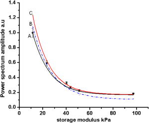

5.

Experiments

5.2.

Intensity Autocorrelation Measurement

The intensity autocorrelation of transmitted photons through the PVA gel is measured using the setup shown in Fig. 2. Two sets of PVA phantoms of dimensions $10\times 10\times 10\mathrm{mm}$ and $50\times 45\times 15\mathrm{mm}$ are fabricated. The samples for measurement are held in position immersed in water in a glass tank. The water provides an appropriate coupling medium for delivering the US beam into the object. The focusing US transducer is made of piezo-electric transducer (PZT) pasted on a concave block. There is a hole of diameter $2\mathrm{mm}$ in the center of the transducer, which allows the interrogating light from a $\mathrm{He}\text{-}\mathrm{Ne}$ laser to propagate along the transducer axis, also intercepting the focal volume. There is provision also for moving the transducer so that the light propagates perpendicular to the transducer axis, again intercepting the focal volume [Fig. 2b]. The transmitted light is picked up by a single-mode fiber, which ensures a high signal-to-noise ratio in the detected current by picking up a single speckle for the photon counting detector. The photon counting system is a single unit with a photomultiplier tube (PMT) and a pulse amplifier discriminator (PAD) (Hamamatsu Photonics K.K., Hamamatsu City, Japan, H7360-03). The output from the photon counting unit is given to an autocorrelator (Flex, Bridgewater, NJ, 021d),²⁷ which helps us get the intensity autocorrelation $g_2\left(\tau \right)$ of the exiting photons from the phantom. The correlator output is Fourier transformed and the power spectral density at $1\mathrm{MHz}$ is measured by finding the area under the peak at $1\mathrm{MHz}$ , which is proportional to the modulation depth in $g_2\left(\tau \right)$ . In this experiment we wanted to ascertain how this depth of modulation varied when ${\mu }_a$ and $G^{\prime }$ of the material of the phantom are varied.

For this purpose we have used sets of PVA gel slabs with ${\mu }_a=2.5\times {10}^{-4}{\mathrm{mm}}^{-1}$ (negligibly small absorption, which was obtained without adding India ink while the gel was being set), $4.4\times {10}^{-2}{\mathrm{mm}}^{-1}$ and $6\times {10}^{-2}{\mathrm{mm}}^{-1}$ . Each of these sets with a particular value of ${\mu }_a$ contained samples, prepared using the recipe given in Ref. 23, with $G^{\prime }$ given by $11.39\pm 0.81$ , $23.42\pm 0.82$ , $40.35\pm 1.34$ , $43.73\pm 0.41$ , $51.18\pm 0.82$ , and $97.28\pm 1.23\mathrm{kPa}$ . These $G^{\prime }$ values are also verified by independent measurements.²³ Using the previous set of phantoms, the modulation depth in $g_2\left(\tau \right)$ was measured, from the power spectral amplitude at $1\mathrm{MHz}$ , for both the axial and transverse illumination of the phantom. A typical experimental power spectrum obtained from an axial measurement is shown in Fig. 6 . The detection noise around $1\mathrm{MHz}$ , seen in the power spectrum as the noise pedestal, is quite small compared to the signal strength at $1\mathrm{MHz}$ .

Fig. 6

A typical experimentally obtained power spectrum, showing the noise levels at the ultrasound frequency. This is obtained from an axial measurement, using the small phantom described in the experiments, corresponding to a storage modulus of $11\mathrm{kPa}$ . The amount of shot noise level is very small with a pedestal of 0.3, compared to the maximum of 17.14 at $1\mathrm{MHz}$ .

The variations of power spectral amplitude with storage modulus are plotted in Figs. 3 and 4, which also compare the experimental variations with theoretically obtained variations. All the previous results are corresponding to experiments and simulations done on the smaller object. The same experiments are repeated with the larger object as well. Variations of the measured power spectral amplitude, from the axial photons, with storage modulus and absorption coefficient, shown in Fig. 4b, are similar to the corresponding results for the smaller object shown in Fig. 4a. For the larger object, owing to the increase in ${\mu }_s$ with storage modulus of the phantom, the light output became very poor beyond the storage modulus value of $50\mathrm{kPa}$ , and the intensity autocorrelation could not be measured beyond this stiffness. The results are further discussed in the next section.

6.

Results and Discussions

Figure 3 compares the experimentally measured variation of modulation depth $M$ with the corresponding theoretically arrived-at values. Curve A is the variation of $M$ with storage modulus, when ${\mu }_a=2.5\times {10}^{-4}{\mathrm{mm}}^{-1}$ , and the interrogating light is along the US transducer axis. Since the amplitude of oscillation of particles in the focal region is along the mean direction of light propagation, and since this amplitude is inversely related to $G^{\prime }$ , the local storage modulus of the medium, there is a sharp decrease in the phase modulation picked up by the interrogating light in this case. This can be compared to curve B, which shows the $g_2\left(\tau \right)$ modulation depth similar to curve A but for light launched perpendicular to transducer axis. Since the vibration amplitude is axial, the phase modulation picked up by the light launched in the transverse direction and diffusing through the insonified region is very small. This causes a relatively smaller modulation in the measured $g_2\left(\tau \right)$ and a smaller variation of this modulation with storage modulus of the insonified region. From curve B it is seen that 1. the experimentally measured variation agrees well with the theoretically arrived-at variation in the modulation depth, and 2. beyond a storage modulus of $\sim 30\mathrm{kPa}$ , the modulation depth did not change appreciably with further increase in storage modulus. Further, for the radiation force applied from the transducer employed in the experiments, both the curves merge to give the same pedestal value of the modulation depth, for storage modulus beyond $80\mathrm{kPa}$ . This pedestal value of modulation depth, which remained invariant with further increase in local storage modulus, should be the contribution solely from $\mathrm{\Delta }n$ , i.e., through the ${\sum }_j\mathrm{\Delta }{n}_j{\ell }_j$ term of Eq. 7. The interaction length of the axial and transverse directed photons in the US focal region is approximately of the ratio 4:1. In spite of this, the residual modulation depth owing to $\mathrm{\Delta }n$ approached the same pedestal value, because of the inherent insensitiveness of the diffusing wave spectroscopy (DWS) probe to pick up path length variation beyond one wavelength of the interrogating light. This constant modulation depth, which is the contribution of refractive index modulation, can be subtracted from the set of measurements of curve A, to arrive at the modulation depth owing to the displacement of particles alone.

Figure 4 plots the variation of $M$ in the case of simulation and experiments with storage modulus, with ${\mu }_a$ as a parameter for ${\mu }_a=2.5\times {10}^{-4}$ , $4.4\times {10}^{-2}$ , and $6\times {10}^{-2}{\mathrm{mm}}^{-1}$ . Figure 4a corresponds to experiments and simulations done on the smaller object, whereas Fig. 4b is for the larger object. In both the cases there is close agreement between experimental variation and those predicted through simulations. The variation of the power spectral amplitude with storage modulus is both sharp and nonlinear when the interrogating light is along the US transducer axis. They tend to attain a constant value beyond a certain storage modulus, which in our experiments and for the transducer used was $80\mathrm{kPa}$ . As seen from Fig. 3, this contribution is the same for both axial and transverse interrogation. In Fig. 4b as mentioned earlier, the experimental measurement of $g_2\left(\tau \right)$ was limited to $40\mathrm{kPa}$ only, because of lack of the adequate number of exiting photons.

If we assume that the change in $\mathrm{\Delta }n$ with storage modulus is negligible, the contribution to $g_2\left(\tau \right)$ modulation from refractive index fluctuation is the same for all measurements for an object of a particular absorption coefficient, which is the pedestal value to which the measurements approach as the storage modulus is increased. For the sample with ${\mu }_a=2.5\times {10}^{-4}{\mathrm{mm}}^{-1}$ , this value is approximately 0.2, which can be subtracted from the other measurements in the set to give the contribution from amplitude of vibration alone.

From curve B of Fig. 3, we see that for transverse interrogation, the variation in the measured modulation depth with storage modulus is not significant. Therefore, in an object that has both absorption coefficient and stiffness variation, the modulation depth measured from transverse photons with focused US insonification can be used to get a fairly accurate estimate of the absorption coefficient variation, without the storage modulus variation significantly affecting the measurements. Therefore, in UAOT, for a possible quantitative reconstruction of ${\mu }_a$ variation, transverse read-out is the most appropriate.

The PVA phantom, because of the process used to manufacture the polymer gel, cannot have its storage modulus varying independent of its scattering coefficient. This need not be true in practical situations where malignancy presents increased stiffness and absorption coefficient and not a large variation in scattering coefficient. Curve A of Fig. 5 compares the experimental variation of $g_2\left(\tau \right)$ modulation with stiffness with theoretical simulation data, wherein ${\mu }_s$ varies with stiffness similar to that seen in the phantom. The experimental variation fits very well with the corresponding theoretical variation in curve A. Curves B and C are variations of the simulated $g_2\left(\tau \right)$ modulation depth with storage modulus, with the ${\mu }_s$ used as a parameter. These do not quite agree with the experimental measurements. These curves tell us that the scattering coefficient variation does contribute to the modulation depth in $g_2\left(\tau \right)$ but by a very small amount.

7.

Conclusion

The present work is aimed at pushing the case for a quantitative reconstruction from ultrasound assisted optical elastography (UAOE).¹⁵ In UAOE, the read-out is the modulation in $g_2\left(\tau \right)$ , which originates from the optical path length modulation created by the US beam in the focal region. Since storage modulus is to be recovered from the amplitude of vibration induced by the US force, it is important for the quantitative recovery of storage modulus to separate the contribution of $\mathrm{\Delta }n$ to the modulation in $g_2\left(\tau \right)$ . In the present work it is shown that the displacement induced by the US force in the focal region is along the axis of the transducer, and the fluctuations in refractive index are not direction dependent. We show here that the modulation in $g_2\left(\tau \right)$ read-out from the light propagation perpendicular to the US transducer axis is not significantly affected by the storage modulus variation, whereas for axial light propagation, the storage modulus variation has a significant effect on the read-out. The modulation depth decreases and converges to a constant value as the storage modulus increases beyond a certain value. This constant modulation depth is the contribution of only refractive index fluctuation, and was the same for both axial and transverse photon interrogation. From this it is possible to quantify and remove the contribution to the measured $g_2\left(\tau \right)$ modulation from the refractive index fluctuations. In addition, we have found that the ${\mu }_a$ contrast, as read-out from the $g_2\left(\tau \right)$ modulation depth of axially directed photons, is severely affected by an increase in storage modulus. But for transverse directed photons, the ${\mu }_a$ contrast is not seriously affected by an increase in storage modulus and therefore, for the reconstruction of absorption coefficient in UAOT, the light should be launched perpendicular to the focusing US transducer axis. Finally, it is also seen that contribution to the modulation depth through ${\mu }_s$ variation is not very significant.