1.

Introduction

Osteoarthritis (OA) is the most common joint problem worldwide and is estimated to affect nearly 60 million Americans. Although a number of factors contribute to its development, including obesity, trauma, and genetic predisposition, the hallmark of osteoarthritis is progressive damage to articular cartilage.¹ This specialized cartilage, found at the articular surface of diarthrodial joints, consists of chondrocytes imbedded within a matrix of collagens, proteoglycans, and proteinases, and provides a smooth, low-friction surface for movement. As damage progresses, the chondrocytes lose their ability to synthesize a high-quality matrix. Fissuring of the articular cartilage can result in fragmentation and deposition of small loose bodies within the joint space. Typically, a low-grade inflammatory reaction occurs, and the synovial fluid may lose some of its normal viscoelastic and lubricating properties. Subchondral bone becomes exposed and results in sclerosis. In response to these stresses, there is typically new bone formation, termed osteophytes, which are preferentially found at the joint margins. Classically, OA is most often found in the large weight-bearing joints of the lower extremities, particularly the knees and hips. However, there is also a subset of individuals with a predilection for developing OA of the hands and a more generalized form of OA.² Interestingly, it is the distal and proximal interphalangeal joints that are most often affected and culminate in the development of Heberden’s (distal) and Bouchard’s (proximal) nodes.

Although current therapy is symptomatic, remarkable advances have been made in our understanding of the pathophysiology of OA.^{3, 4, 5} Much of the degradation of cartilage is mediated through matrix metalloproteinases, and the development of small-molecule inhibitors has been an area of active research interest.^{6, 7, 8} In anticipation of the development of new products with the potential to alter the natural history of OA, it will be crucial to have noninvasive technologies that can detect early OA and monitor efficacy of therapy.

To diagnose cartilage abnormalities and alterations in composition of synovial fluid in joints affected by OA, a variety of imaging methods have been developed and tested, such as radiography (x-ray), ultrasound (US), computed tomography (CT), and magnetic resonance imaging (MRI).^{9, 10, 11, 12, 13} Of all of the imaging modalities, the best established is x-ray. However, while plain radiographs are able to visualize joint space narrowing and osteophyte formation, they are insensitive to changes in cartilage and fluid and therefore incapable of capturing the primary features of the early stages of OA.¹⁴ MRI, another commonly used modality in clinical practice, can reliably detect early OA when high contrast agents are used. However, it is costly and time consuming.¹⁵ Computed tomography (CT) has also been employed in the diagnosis of OA. However, it too is very expensive and provides only qualitative structural information in severe OA.⁹ Musculoskeletal ultrasound has been the subject of much recent interest in evaluating rheumatoid arthritis and regional musculoskeletal pathology.^{8, 10, 16, 17} A strongly operator-dependent modality and sensitive only to changes in the boundary layer, it has limited utility in evaluation of the early stages of OA, at a time when there has been little change in joint space.¹⁸

As an emerging nonionizing technology, near-infrared optical imaging has received much attention because optical techniques offer unique advantages over the existing imaging methods mentioned. Optical imaging is low in cost and noninvasive. Besides the advantages of utilizing only low-level and nonionizing near-infrared radiation, it can be realized in compact, portable instruments. Moreover, the imaging contrast offered by diffuse optical tomography is high, suggesting a possible use in early OA detection. Ultimately, optical imaging methods are able to provide a variety of functional and structural information with high sensitivity and specificity compared to other imaging modalities. This is especially true for the joints of the fingers, where the small dimensions and much higher transmitted light intensities should result in better signal-to-noise ratios and greatly improved spatial resolution.

Three typical optical techniques are currently being used for optical tissue imaging: continuous-wave, time-resolved, and frequency-domain methods. Most of these studies have been focused on direct image formulation from the measured optical data, which may not fully exploit all of the information provided. In consideration of the advantages over direct imaging methods, several groups are now concentrating on model-based diffuse optical tomography (DOT) methods,^{19, 20, 21} in which the diffusion approximation to model light propagation in tissue is used for multiply scattered light. Due to the use of an effective reconstruction algorithm, DOT is able to improve the resolution limitation and to detect deep tissues. Phantom and clinical experiments have shown that the diffuse optical reconstruction method is able to recover both structural and functional information from brain and breast tissues.¹⁹ Recent phantom and clinical studies showed that DOT can also provide quantitative images of joints and associated bones.²² For example, Xu, Iftimia, and Jiang²³ first reported the DOT imaging of healthy finger joints. Schwaighofer, ²⁴ Scheel, ²⁵ and Hielscher ²¹ demonstrated that optical tomography could be used to detect and quantitate the degree of inflammation within the finger joints of individuals with rheumatoid arthritis. Studies have indicated that the optical properties of healthy and diseased joint tissues are quite different.^{26, 27} The goal of this work is to describe an integrated 3-D DOT imaging system and reconstruction algorithm that has the potential to monitor and diagnose early osteoarthritis based on our previous phantom and in-vivo experiments.^{20, 23}

In this study, we demonstrate that DOT imaging could distinguish between normal and degenerative joints. Besides the introduction of the imaging measurement system and reconstruction algorithm, we discuss in detail the radiographic appearance of two patients with OA and three healthy volunteers, based on qualitative optical images and quantitative optical properties. Moreover, we measured the thickness of cartilage and fluid in the distal interphalangeal (DIP) finger joint using a fitting method, which provides the structural size information to detect early changes of OA. Finally, the optical tomography images are also compared with x-ray findings.

2.

Experimental Materials and Methods

2.1.

Optical Imaging

All the experiments with human subjects were performed by our recently developed multichannel (64 sources and 64 detectors) photodiodes-based DOT system,^{28, 29} shown in Fig. 1 . The system consisted of laser modules, a hybrid light delivery subsystem, a fiber optics/tissue interface, light detection modules, and a data acquisition module.

Fig. 1

Photograph of the DOT imaging system. The insert is a close-view photograph of the finger/coupling medium/fiber optics interface.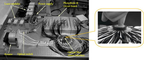

While the system has eight diode lasers (B&W TEK Incorporated, Delaware and Power Technology Incorporated, Arkansas) with wavelengths from $634\text{to}974\mathrm{nm}$ acting as light sources, this study was based on the laser at $853\mathrm{nm}$ with a maximum output of $210\mathrm{mW}$ . The light intensity was measured as $70\mathrm{mW}$ when it was delivered to the fiber optical interface, and further reduced to $10\text{to}30\mathrm{mW}$ at the surface of the finger, which depended on the location of the finger relative to an excitation source position. An efficient and low-cost hybrid subsystem that included a $1\times 8$ optical switch (VX500, Dicon Fiberoptics Incorporated, California) and a motorized rotator (RT-5-M17, Newmark Systems Incorporated, California) was designed to deliver laser light to excitation points on the fiber optics/tissue interface. The motorized rotator drove an optical fiber, called a laser source fiber (LS fiber), to 64 positions to transfer the light beam into 64 source fiber bundles ( $1\mathrm{mm}$ in diameter, 0.55 NA, RoMack Incorporated, Virginia) that were circularly arranged. At each position, light from the laser module was coupled into the LS fiber via the optical switch.

A cylindrical fiber optics/tissue interface was employed in our study, where 64 source fiber bundles and 64 detector fiber bundles ( $2\mathrm{mm}$ in diameter, 0.55 NA, RoMack Incorporated, Virginia) were positioned in four layers with a $5.0\text{-}\mathrm{mm}$ distance between two adjacent layers. In each layer, 16 source fiber bundles and 16 detection fiber bundles were alternatively placed with $11.25\mathrm{deg}$ intervals. A total volume with $15\mathrm{mm}$ height and $30\mathrm{mm}$ diameter was covered by these four layers, and the subject’s finger joints were located inside it. To hold the finger as well as satisfy the diffusion equation, the space between the finger and the plexiglas wall that was used to hold the source/detector fiber bundles was filled with a tissue-like phantom made from water, agar, Indian Ink, and Intralipid (Fig. 1). This tissue-like medium can be solidified when its temperature is under $40°\mathrm{C}$ . After the subject placed her/his finger into the cylinder, the medium was poured in and quickly solidified within a couple of minutes. The phantom materials were chosen so that the optical properties (especially the absorption and scattering coefficients) of these phantoms were close to those of soft tissue in human fingers. Here the absorption and scattering coefficients of the phantom were $0.014∕\mathrm{mm}$ and $1.0∕\mathrm{mm}$ , respectively.

We chose 64 low noise integrated silicon-photodiodes (S8745, Hamamatsu, New Jersey) for parallel signal collection. A total of four homemade programmable circuit boards controlled all of these detector units, which were mounted into four metal boxes. The electric noise level of each sensor unit was $1.0\mathrm{mV}$ . For the wavelength range of $634\text{to}974\mathrm{nm}$ , the sensitivity of the S8745 silicon photodiode was between 0.34 and $0.52\mathrm{V}∕\mathrm{nW}$ , and the noise equivalent power of this system was calculated to be $2.9\text{to}1.9\mathrm{pW}$ . The four gain levels for each detector unit was automatically selected via a PCI-DDA02/12 output board (Measurement Computing, Massachusetts) and therefore the dynamic range of the measurement had been extended to $2.7\times {10}^8$ . Data acquisition was performed via a single $16\text{-}\text{bit}$ A/D board with a $200\mathrm{kS}∕\mathrm{s}$ maximum ADC rate (PCI-DA6035, Measurement Computing, Massachusetts). Data acquisition from one and eight wavelengths took about 5 and $27\text{minutes}$ , respectively. The system was also carefully calibrated through a two-step calibration procedure.³⁰ An IBM Pentium 4 PC controlled the whole DOT system utilizing the LabView program. The optical switch and the motorized rotator were controlled through the parallel port and RS232 serial port, respectively.

2.4.

Patient Examinations

Five persons including two patients and three healthy volunteers were recruited from the hospital and university campus. The clinical study was approved by the University Institutional Review Board, and the volunteers gave informed consent prior to investigation. All the diseased joints were examined by a physician and showed clear signs of OA. For the two patients we scanned, they had difficulty in moving their fingers smoothly and suffered from pain within their finger joint during movement. Their situation went worse in cold weather. Joint space narrowing was clearly observed.

The reconstruction of the DIP joint with the coupling phantoms ( $30\mathrm{mm}$ in diameter and $20\mathrm{mm}$ in height) was performed with a mesh of 3009 nodes and 12,800 tetrahedral elements. 64 sources and 64 detectors were distributed uniformly along the surface of the phantom at four planes ( $z=2.5$ , $z=7.5,z=12.5$ , and $z=17.5\mathrm{mm}$ ; 16 sources and 16 detectors at each plane). The initial guesses used for the reconstruction were ${\mu }_s^{\prime }=1.0∕\mathrm{mm}$ , ${\mu }_a=0.03∕\mathrm{mm}$ , $S=9.8$ , and $\alpha =0.001$ . The reconstruction took about $2\mathrm{h}$ on a $1\text{-}\mathrm{GHz}$ Pentium 4 PC with about 20 iterations.

Because structural size information is also an important measure of the degree of OA,^{37, 38} besides the recovered optical properties, a novel fitting algorithm is developed to assess the thickness of cartilage and synovial fluid from DOT imaging in consideration of the following points: 1) the gradient for image intensity exists between the bones and joint tissues; 2. the fluid thickness is much thinner than the cartilage; 3. it only makes sense for computing average thickness of gap and cartilage tissues because joint thickness is position dependent. The proposed fitting algorithm, called the full-width at 30% maximum (FW30%M) method, was able to calculate the quantitative structural size of joint tissues.

For the FW30%M method, we first took six representative dorsal and coronal slices (three $x\text{-}z$ slices and three $y\text{-}z$ slices) from the reconstructed 3-D image for quantitative analysis, which included two central slices in dorsal and coronal planes, respectively. The six slices chosen were different for each patient. For instance, for OA patient 1, the three dorsal slices were taken at $y=-1,0$ , and $1\mathrm{mm}$ , and the three coronal slices were taken at $x=-3,-1$ , and $1\mathrm{mm}$ . The distance between two adjacent slices was about $1\text{to}2\mathrm{mm}$ . While the central dorsal and coronal slices go from $-15\text{to}15\mathrm{mm}$ , the width of the other four slices is smaller than that of the central ones.

For each slice, we plotted five central lines for quantitative analysis of absorption and scattering properties, as shown in schematic Figs. 2a and 2b . We limited the five lines within the finger domain. These lines were not always vertical, and for some cases we used lines that were tilted and parallel to the middle line of the bones. Thus we were able to ensure that the schematic curves shown in Fig. 2c really represented actual slices from the side-to-side 2-D images. The full width at 30% maximum curve for each line was divided into three parts: bone, cartilage, and fluid. The interface points among bone, cartilage, and fluid were taken as 30% of the nearest highest values on the curves, as shown in schematic Fig. 2c. In this study, quantitative analysis was conducted for 30 central lines located on six slices of each recovered 3-D image. By using this threshold, we calculated the mean thickness of cartilage as well as fluid, and we also provided the averaged optical properties of bone, cartilage, and fluid. The quantitative results for the scattering coefficients were given in Table 1 and the absorption properties are listed in Table 2 . Further, it should be noted that for the developed fitting algorithm we used the joint space measured from the x-ray images of healthy joints as the standard to determine the criteria value for estimating the geometrical sizes of joint tissues from the optical images. We found 30% at maximum gave us the best results relative to x-ray. Additionally, the difference between different slices surely existed, but we calculated the mean values of different slices to reduce the error. Finally, the mean structural sizes of joints from the high-resolution x-ray images were provided in Tables 1, 2 for comparison.

Fig. 2

(a) 3-D schematic of the finger joint measurement configuration. (b) Schematic of 2-D dorsal/coronal slice along with the five lines used for quantitative analysis. (c) Schematic of a 2-D optical property profile along line AB shown in (b). $V_{a,b,c}$ indicates optical property value at different points along the profile.

Table 1

Reconstructed scattering related parameters for five cases. Note that ua−c , ua−f , and ua−b are the absorption coefficients of cartilage, fluid, and bone, respectively. us−c′ , us−f′ , and us−b′ are the scattering coefficients of cartilage, fluid, and bone, respectively.

	Case	Jointtissues	Averaged us′ (1∕mm)	Meanthickness(mm)	X-raysize(mm)	us−c′∕us−b′	us−f′∕us−b′
OA	1	Bone	2.30	N/A	N/A	0.843	0.796
		Cartilage	1.94	1.0	0.75
		Fluid	1.83	0.3	N/A
	2	Bone	1.67	N/A	N/A	0.719	0.599
		Cartilage	1.20	1.1	0.78
		Fluid	0.99	0.4	N/A
Healthy	3	Bone	1.96	N/A	N/A	0.622	0.469
		Cartilage	1.22	1.7	1.46
		Fluid	0.92	0.6	N/A
	4	Bone	1.51	N/A	N/A	0.675	0.536
		Cartilage	1.02	1.7	1.21
		Fluid	0.81	0.6	N/A
	5	Bone	1.45	N/A	N/A	0.666	0.531
		Cartilage	0.97	1.9	1.42
		Fluid	0.77	0.6	N/A

2.4.1.

Case 1: osteoarthritis patient 1

This patient was a $50\text{-}\text{year}$ -old female, who was first diagnosed with OA in both joints of the index finger about $10\text{years}$ ago. Figures 3a and 3b plot the longitudinal scattering slices (along both $x$ and $y$ coordinates) of a recovered 3-D image for patient 1. Figures 3c and 3d display the reconstructed longitudinal absorption slices for this patient. The x-ray findings are given in Fig. 3e. The 3-D tomosynthesis x-ray image is also given later for case 1 to show the exact position and orientation of the joint. The structural size of the joint, including the fluid and cartilage, is calculated and listed in Tables 1, 2, where the average optical properties of bone and cartilage as well as fluid are also provided.

Fig. 3

Reconstructed images at selected dorsal/coronal planes for case 1: (a) scattering slices at $y=-2,-1.5,-1,-0.5,0,1,2$ , and $2.5\mathrm{mm}$ (dorsal planes); (b) scattering slices at $x=-5,-4,-3,-2,-1,0,1$ , and $2\mathrm{mm}$ (coronal planes); (c) absorption slices at $y=-2,-1.5,-1,-0.5,0,1,2$ , and $2.5\mathrm{mm}$ (dorsal planes); (d) absorption slices at $x=-5,-4,-3,-2,-1,0,1$ , and $2\mathrm{mm}$ (coronal planes); and (e) x-ray image. The axes (left and bottom) indicate the spatial scale in millimeters, whereas the color scale gives the absorption or scattering coefficient in inverse millimeters.

2.4.2.

Case 2: osteoarthritis patient 2

The second patient was also a $50\text{-}\text{year}$ -old female, whose DIP joint developed clinical OA about $4\text{years}$ ago. Figures 4a and 4b plot the recovered scattering slices of the 3-D image for this patient. Figures 4c and 4d provide the reconstructed longitudinal absorption slices for the 3-D representation of this joint. We also computed the recovered structural sizes and optical properties of the joint, and these quantitative results are given in Tables 1, 2 for this patient. An x-ray image for patient 2 is presented in Fig. 4e. The tomosynthesis x-ray image for case 2 is provided later.

Fig. 4

Reconstructed images at selected dorsal/coronal planes from case 2: (a) scattering slices at $y=-3,-2,-1,-0.5,0,1,1.5$ , and $2\mathrm{mm}$ (dorsal planes); (b) scattering slices at $x=-1.5,-1,-0.5,0,0.5,1.0,1.5$ , and $2\mathrm{mm}$ (coronal planes); (c) absorption slices at $y=-3,-2,-1,-0.5,0,1,1.5$ , and $2\mathrm{mm}$ (dorsal planes); (d) absorption slices at $x=-1.5,-1,-0.5,0,0.5,1.0,1.5$ , and $2\mathrm{mm}$ (coronal planes); and (e) x-ray image.

2.4.3.

Case 3: healthy volunteers

The ages of the healthy volunteers shown as cases 3 to 5 ranged from 32 to 40. Figures 5a and 5b display the recovered longitudinal scattering slices for case 3. The reconstructed absorption slices are given in Figs. 5c and 5d. The reconstructed mean absorption and scattering properties as well as structural sizes are presented in Tables 1, 2. Moreover, an x-ray image is provided to compare with the optical tomography images for the healthy volunteer, as shown in Fig. 5e. The tomosynthesis x-ray image for case 3 is displayed in Fig. 6c , cases 1 and 2 in Figs. 6a and 6b, respectively.

Fig. 5

Reconstructed images at selected dorsal/coronal planes from case 3: (a) scattering slices at $y=-3,-2,-1.5,-1,-0.5,0,1$ , and $1.5\mathrm{mm}$ (dorsal planes); (b) scattering slices at $x=-1,-0.5,0,0.5,1.0,1.5,2$ , and $3\mathrm{mm}$ (coronal planes); (c) absorption slices at $y=-3,-2,-1.5,-1,-0.5,0,1$ , and $1.5\mathrm{mm}$ (dorsal planes); (d) absorption slices at $x=-1,-0.5,0,0.5,1.0,1.5,2$ , and $3\mathrm{mm}$ (coronal planes); and (e) the x-ray image.

Fig. 6

Reconstructed 3-D tomosynthesis x-ray images: (a) case 1; (b) case 2; and (c) case 3.

Table 2

Reconstructed absorption related parameters for five cases. Note that ua−c , ua−f , and ua−b are the absorption coefficients of cartilage, fluid, and bone, respectively. us−c′ , us−f′ , and us−b′ are the scattering coefficients of cartilage, fluid, and bone, respectively.

	Case	Jointtissues	Averaged μa (1∕mm)	Meanthickness(mm)	X-raysize(mm)	ua−c∕ua−b	ua−f∕ua−b
OA	1	Bone	0.0526	N/A	N/A	0.859	0.817
		Cartilage	0.0452	1.0	0.75
		Fluid	0.0430	0.3	N/A
	2	Bone	0.055	N/A	N/A	0.836	0.782
		Cartilage	0.046	1.1	0.78
		Fluid	0.043	0.4	N/A
Healthy	3	Bone	0.0513	N/A	N/A	0.657	0.534
		Cartilage	0.0337	1.8	1.46
		Fluid	0.0274	0.5	N/A
	4	Bone	0.0796	N/A	N/A	0.628	0.500
		Cartilage	0.0500	1.3	1.21
		Fluid	0.0398	0.4	N/A
	5	Bone	0.0560	N/A	N/A	0.559	0.414
		Cartilage	0.0313	1.5	1.42
		Fluid	0.0232	0.5	N/A

3.

Discussion

In this pilot clinic evaluation of an optical imaging system for OA of the hand, we obtained two types of imaging parameters, including optical properties and the structural sizes of cartilage and fluid. Physically, these quantitative results represent two different intrinsic properties of the finger joint and can be employed to diagnose and monitor the progression of early OA.

We first examine the qualitative images shown in Figs. 3, 4, 5. From these absorption and scattering images, we immediately note that the bones are clearly delineated (most red color regions) for both OA and normal joints, where we also see that the shape and size of the bones are better recovered in the absorption images than those in the scattering images. While there is no clear boundary between the bones and cartilage/fluid, the joint tissue/space is clearly identified. Here, the joint space narrowing seems apparent for both OA joints (Figs. 3 and 4) relative to the healthy joints (Fig. 5), and this narrowing appears to be stronger for the more advanced OA joint (patient 1, Fig. 3). Importantly, we note that the distributions of both absorption and scattering coefficients in the joint space are highly heterogeneous, especially for the advanced OA joint (e.g., see Fig. 3), while such distributions are quite homogeneous in general for the healthy joints (e.g., see Fig. 5).

We now discuss the quantitative results given in Tables 1, 2. We note from Table 1 that the scattering value of the diseased fluid for both OA cases ( ${\mu }_s^{\prime }=1.83∕\mathrm{mm}$ and $0.99∕\mathrm{mm}$ ) are larger than that of the healthy fluid ( ${\mu }_s^{\prime }=0.92,0.81$ , and $0.77∕\mathrm{mm}$ ), with the advanced OA case having the largest value $({\mu }_s^{\prime }=1.83∕\mathrm{mm})$ . While the scattering coefficient value of cartilage for the advanced OA joint is the largest, we see that this value for OA patient 2 is slightly smaller than that for healthy case 3, but larger than that for other healthy cases. Interestingly, the difference in scattering coefficient of joint tissues between the OA and healthy controls seems apparent from the ratio of this optical property of cartilage and fluid to that of bone (the last two columns in Table 1). We immediately note that this ratio for both diseased cartilage and fluid is larger that that for normal cartilage and fluid. Furthermore, as shown in Table 1, the mean thickness of cartilage and fluid for cases 1 and 2 are 1.0 and $0.3\mathrm{mm}$ , and 1.1 and $0.4\mathrm{mm}$ , respectively. However, the mean thickness of cartilage and fluid for cases 3, 4, and 5, are 1.7 and $0.6\mathrm{mm}$ , 1.7 and $0.6\mathrm{mm}$ , and 1.9 and $0.6\mathrm{mm}$ , respectively. Compared with the normal controls, the two patients with OA appear to show joint space narrowing by our technique.

Similar observations can be made regarding the quantitative results listed in Table 2 for absorption coefficient images. We see from Table 2 that the absorption value of the diseased fluid for both OA cases $({\mu }_a=0.043∕\mathrm{mm})$ is larger than that of the healthy fluid ( ${\mu }_a=0.0274,0.0398$ , and $0.0232∕\mathrm{mm}$ ). We note, however, that the absorption coefficient values of the diseased and healthy cartilages do not show clear differences. Again, we observe that the ratio of the absorption coefficient of the diseased cartilage and fluid to that of associated bone is also larger than this ratio for the normal controls. In addition, as displayed in Table 2, the mean thickness of cartilage and fluid computed from the absorption property distributions are 1.0 and $0.3\mathrm{mm}$ , and 1.1 and $0.4\mathrm{mm}$ , respectively, for cases 1 and 2. However, the mean cartilage and fluid thickness for cases 3 to 5 are 1.8 and $0.5\mathrm{mm}$ , 1.3 and $0.4\mathrm{mm}$ , and 1.5 and $0.5\mathrm{mm}$ , respectively. Judging from the structural size parameters in Table 2, we find that the mean thickness of cartilage and fluid in the joints affected by OA seems to be thinner than healthy ones. We can also see from Tables 1, 2 that the structural size computed from the absorption and scattering distributions are in general consistent with each other, except for case 4. The joint space narrowing observed from the optical images for the OA joints are also consistent with the x-ray findings [Figs. 3e and 4e]. It is noted from Tables 1, 2 that the error of the recovered structural parameters is less than 30% compared to the x-ray findings. Although x-ray imaging is unable to show contrast for soft joint tissues, its high resolution ability for hardware tissue provides a standard for examining the structural information obtained from DOT. In this regard, we can conclude that the optical images presented in Figs. 3, 4, 5 are geometrically consistent with the x-ray images shown in Fig. 6.

It should be noted that although joint space narrowing is an important indicator for OA diagnosis, we cannot judge if this patient is really affected by this disease from only structural information, as natural variations exist between different individuals. Hence, we must employ both structural (space narrowing) and functional information (optical properties) to diagnose OA.

While we are confident about the accuracy of the recovered optical properties of the nonfluid regions, the accuracy of the properties for the fluid may be overestimated. This overestimation could be caused by the breakdown of the photon diffusion equation in the region of fluid, as it is well known that the scattering coefficient needs to be much larger than the absorption coefficient for the diffusion equation to be used accurately. We are currently implementing a 3-D reconstruction algorithm based on higher-order diffusion equations, which should eliminate such errors, as we have shown in 2-D reconstruction.³⁹

In summary, we report the first application of diffuse optical tomography to the assessment of OA in finger joints. OA-induced joint narrowing is fully and quantitatively revealed by the DOT imaging. It is noted from reconstructed results that the optical properties as well as the size between OA and healthy joints are quite different, and both could be used to monitor the progression of early OA.