|
|
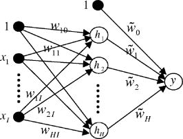
1.IntroductionRecently, laser tweezers and Raman spectroscopy (LTRS) were combined to diagnose single living human cells confined in a laser trap.1, 2 Both solid tumors surgically removed from human colorectal cancer sites1 and human lymphocytes2 were investigated. In the first case, primary culture protocols were followed to detach the cancer cells from their surroundings,1, 3 while in the second case, the healthy and transformed lymphocytes were already in single-cell form. In contrast, DNA flow cytometry (FCM) is a currently adopted medical procedure to evaluate the malignancy of a tumor,4 in which single-cell suspensions are prepared, stained with a DNA-binding fluorophore, and analyzed by a flow cytometer. LTRS and DNA FCM carry several similarities. First, both are single-cell techniques, in which the cells are analyzed one by one; second, both share the same procedure for sample preparation (up to the staining); and third, in both cases, the cells are detected in an aqueous environment involving laser excitation and optical detection. DNA FCM relies on ploidy information, such as irregularities of DNA contents, extra chromosomes, and increased percentage of S-phase cells undergoing DNA replication, to quantitate the aggressiveness of cancer. Thus, it cannot reveal the cell structural changes or the biochemical variations associated with the normal-to-cancer transition. Furthermore, a DNA FCM analysis typically requires 20,000 single cells in order to accumulate enough statistical significance5; therefore, such tests are unavailable to small amount samples from exfoliative cytology or biopsies on small tumors. Last, the accuracy of DNA FCM tests tends to fluctuate on several factors. A procedural guideline has been created to ensure quality control and reproducibility of the test results among different laboratories.5 According to the guideline, adequate neoplastic material in a specimen should be ensured (by other means) before a test can be invoked in order to justify the accuracy. For example, at least 20% tumor cells are necessary if tumor proliferation calculations are needed. Further, accidental mixing with normal tissues can deviate or may even invalidate the test results. The statistical nature of FCM (including conventional FCM) ensures that it is an ensemble averaging technique. On the other hand, LTRS has several characteristics unavailable to DNA FCM. First, LTRS allows single living cells to be directly investigated without any staining, free of the artifacts introduced by the staining process. FCM is essentially a serial method with low efficiency of information, and difficulty in multicolor labeling prevents the simultaneous detection of multiple targets on the same cell, whereas LTRS collects the information about the whole biochemical composition of a cell and reports the contributions of vast chemical function groups in parallel. The abundance of information makes LTRS a true single-cell diagnosis technique, in which the decision is made on each cell, not the ensemble average over 20,000 cells. For the diagnosis of a patient, 20 cells are sufficient for an LTRS test.1 Therefore, small tumor biopsy, exfoliative cytology, and scrape and brush cytology can all be employed to collect materials enough for an LTRS run. Nevertheless, DNA FCM and LTRS are both achievements of laser technologies, and each has its own merits and should be used to supplement each other to assist doctors in the fight against cancers. For two decades, Raman spectroscopy has demonstrated diagnostic power over many diseases, from various cancers, 6, 7, 8, 9 to atherosclerosis,10 to Alzheimer’s disease,11 etc. In the area of cancer studies, great efforts have been taken to obtain the Raman features of lesions from breasts,6, 7 bladders,8 skins,9 etc. Sophisticated diagnostic algorithms have been developed to differentiate, classify, and stage tumors. Over the years, progress in data collection schemes and spectral analysis methods has achieved high accuracy and pushed the detection limit to early stages. As is well known, more than 85% of all cancers originate from the epithelia lining the internal surfaces of human organs. At early stages of cancer development, it is the surface tissue layer that carries diagnostic information, while the underlying bulk tissues are mostly irrelevant and even interfere with the detection. In addition, tissue components in the bulk are the major sources of fluorescence background that complicates the analysis of Raman spectra. In recent years, there is a trend to go from bulk-tissue spectroscopy to surface-tissue spectroscopy. Polarization gating has been exploited to selectively detect the photons singly backscattered from the surface layer within the depth of one scattering length.12 A natural step further would be to retrieve single cells from the epithelium by medical cytology means and study them in isolation from the bulks. This not only creates a disease-screening tool, but also allows investigation on the cell dynamics of carcinogenesis in a controlled environment. LTRS is a way of realizing these new ideas.1, 2 Unfortunately, current LTRS research mainly focuses on bacteria,13, 14 because the primary culture techniques are unfamiliar to the optical community and human cells are larger and harder to trap. Here we call for attention to LTRS research on cancers. Successful Raman diagnosis also depends on spectral analysis. Visual inspection of Raman peaks for clues is subjective, correlations among multiple peaks are often hidden, and simple peak ratios inevitably overlook the overall spectral shape as well as fine spectral details. Sophisticated diagnostic models always resort to some kind of numerical algorithms. Principal component analysis (PCA) is commonly employed to reduce data dimensionality; linear regressions or logistic regressions are the prevailing algorithms for classification. The role of individual Raman peaks in the classification, i.e., which peak is important and which is not, is qualitatively argued (but not quantitatively evaluated) by visual inspection of the spectral patterns of the principal components (PCs) included in the regressions.1, 7 Recently, fittings of the tissue/cell spectra have been attempted, using the spectra of major chemical constituents as the expansion basis.6, 15 However, this method seems oversimplifying, since a cell easily contains at least 8,000 different proteins and many other components. The incompleteness of the spectral basis set can impose a problem to the validity of the results. At the least, some fine structures of the Raman data could be missing in the base spectra and thus ignored in the fitting. In addition, the results can be prone to distortion due to the dominance of one or two strong Raman constituents. Artificial neural network (ANN) is a nonlinear, multidimensional model capable of classifying spectral data.9, 16 The flexibility of ANN results in better discriminating power than any other regression models. But the nonparametric black-box nature of ANN has prevented its adoption compared with other explicit algorithms. To overcome this problem, Sigurdsson invoked sensitivity analysis in their ANN study of skin cancers,16 in which the contribution of each Raman frequency to the network output was numerically evaluated by a function called a sensitivity map. In this paper, we report an LTRS investigation on colorectal cancers and the ANN classification and sensitivity map analysis of the data. Characteristic bands identified by the sensitivity map are linked to intracellular biochemical alterations. The diagnostic relevance of these bands is further studied by Student’s t-tests. 2.Methods2.1.Sample PreparationThis study was approved by the Institutional Review Board of the Cancer Hospital of Fudan University. Written informed consent was obtained from each patient. A total of ten patients with sporadic colorectal adenocarcinomas were involved, including seven males and three females, all Asians, at ages from 33 to 79 with an average of 57.1. Tissue specimens were obtained by surgical resection from the patients. From each patient, the adenocarcinoma and a small amount of normal mucosa adjacent to the tumor site (with separations) were removed. Histological assessments reported no tumor cell infiltration in all the normal mucosa sections. Upon removal, single-cell suspensions were prepared from small portions of the tissue specimens following primary culture protocols.3 Details of the processing procedure were described previously.1 Two suspensions were produced for each patient, one from the tumor and the other from the normal. Histopathology analyses were conducted on the tissue specimens by two pathologists working independently. Only the cases in which consensus was reached are included in the following study. The pathology conclusions serve as the golden standard for the training and testing of ANN. The training set comprises seven moderately-differentiated cases and one poorly-differentiated case, and the test set comprises two well-differentiated cases. 2.2.LTRS Data Collection on Single Living CellsData were acquired by using an LTRS system described previously.1, 17 Briefly, the excitation beam of a diode laser (wavelength ) was delivered into the back pupil of the objective ( immersion) of a Nikon TE2000U differential interference contrast microscope. A laser trap was formed at the focal point. The excitation power was , measured near the focal point. Single-cell suspensions were analyzed in the sample chamber mounted on the microscope stage. Single living epithelial cells were selected, captured, transferred to clear regions, and measured. The measurement of a cell comprised a 60-s signal integration and a 60-s background integration with the cell captured and released, respectively. Their difference was recorded as the raw data signal , with the Raman shift. A total of 20 cancer cells and 20 normal cells were measured for each patient. The ten patients were divided into two groups according to the time sequence of their medical operations: data from the first eight were used to train the ANN, while data from the last two were used for testing. This generated a training set of 160 cancer and 160 normal cells and a test set of 40 cancer and 40 normal ones. Figure 1 presents the average spectra [cancer (curve ); normal (curve )] of the training set and their differences (curve ). 2.3.Diagnostic Modeling by Neural Network Approach2.3.1.PCA reduction of spectral dataPrincipal component analysis is commonly used to reduce data dimensionality. The first step of PCA is a normalization of every spectrum in order to cancel out an overall factor caused by the fluctuation of excitation power. In our PCA, each spectrum was treated as an -dimension vector, where is the total number of pixels. Hence, a unit-vector normalization scheme was adopted,18 i.e., The PCA performed on the 320 spectra in the training set revealed that the first 12 PCs account for 80% of the total variations. Each spectrum from Eq. 1 was then converted to the scores of corresponding PCs formulated aswhere , with index denoting different cells of the set. In Eq. 2, the subscript denotes the individual pixel of a spectrum, while the subscript denotes the score. In PCA, the total number of scores equals the total number of pixels, but only the first tens of scores are useful. To facilitate network training, the scores of the training data were further rescaled to zero mean and unit variance, i.e.,where and .2.3.2.Neural network architectureThe ANN we employed is a two-layer feedforward network with backpropagation training. The network architecture is depicted in Fig. 2 and belongs to the perceptron category. The open circles labeled with or represent the neurons, while the solid circles labeled with represent the inputs to the network. The two circles labeled with “1” are plotted in order to treat the biases in the same fashion as the weights. The network architecture is uniquely defined by the arrangement of the neurons and their interconnections. Each neuron can have multiple inputs but only one output. Each arrow into a neuron represents an input, and the arrow out represents the output. Each interconnection between two nodes is associated with a factor , called weight. For example, the arrow linking to carries a weighting factor , which means that the contribution of to the input of neuron is [Eq. 6, shown later]. The nodes stacked on the left serve as the inputs to the network, and their values are substituted with the scores from Eq. 3. The neurons stacked in the middle form the hidden layer, and the neuron on the right denotes the output layer. The numerical outputs of the neurons and neuron are given by Eqs. 6, 7 later, respectively. Here, the output layer is set to one single node, since a cell is classified as either normal or cancerous. So our network is essentially a binary neural classifier (with modifications described later). The number of nodes in the input column and the hidden layer were determined in the training session by trial and test. Best results were achieved at and . The extreme flexibility of multilayer perceptron networks to approximate arbitrary complex posterior probability functions calls for special procedures to avoid overfitting and detect outliers. Outliers are data points that have been assigned to a wrong category of patterns in the original data set. They are defects of the experimental data. For example, if a cell in the training set is truly normal, but instead determined as cancerous by pathology, then it is an outlier, or vice versa. The existence of outliers is an outcome of the imperfectness of data collection. In our experimental data, the pattern of a cell was set to the pathological classification of the tissue from which the cell was harvested: if the tissue was normal, the cell was normal, or vice versa. However, there was a small possibility that a cell inside a malignant tumor was actually normal, but erroneously labeled as cancerous based on the histopathology grading on the tumor tissue, resulting in an outlier. Outliers in the training set can significantly shift the decision plane of the network if uncorrected and consequently affect the accuracy of network predictions. An outlier probability was introduced in Ref. 16 to correct the classification flipping due to the existence of outliers. In our binary case, this means that where and are the posterior probability for cancer (class 1) and normal (class 0) at the absence of outliers, respectively and and are the actual posterior probability for cancer and normal, respectively. Here the term “posterior” means post-experiment, and the posterior probability is the conditional probability of the cell’s classification under the requirement that it has the characteristics to produce Raman spectrum . Both and contain two terms, indicating that the cell data carry probability of not being an outlier and probability of being an outlier. After straightforward calculations, Eq. 4 can be simplified towhere . The connection of Eq. 5 to the ANN output (Fig. 2) is through .In ANN, the response (the output) of a neuron to the stimuli (the inputs) is calculated through its activation function. In Fig. 2, the activation functions are hyperbolic tangent for the hidden layer, i.e., and linear for the output layer, i.e.,where and are the input-to-hidden weight and bias, and and are the hidden-to-output weight and bias. The ANN estimate to the posterior probability without outlier corrections is predicted asConsequently, the ANN estimates to Eq. 5 become2.3.3.Input-output and training of the networkThe training set comprises the cell data of eight patients, , with the rescaled scores in Eq. 3, and the target value defined as The procedures of Ref. 16 were executed to train the network, but with some modifications. The network optimization was done by minimizing a cost function redefined aswhereandThe first term on the right side of Eq. 11 is the cross-entropy error function, while the second one is a weight-decay regularization to restrict network overfitting on the input noise. The weight vector is a simplified notation for all the network weights and biases, i.e., and its dimension . It is worth pointing out that Eq. 11 is different from the special case of in Ref. 16 for several reasons, where is the number of output classes. The first is that our case employs only one instead of two sets of hidden-to-output weights, so the network is simpler and the dimension of smaller; the second, in Eq. 12 is calculated using the logistic function, while in Ref. 16, the softmax function is used and the two calculated posterior probabilities are not independent, inducing problems in the evaluation of the inverse Hessian and causing a singularity of at . Indeed, our numerical computations confirmed that Eqs. 11 to 13 produce better training results than the version of Ref. 16.The unknown parameters are the network weights-biases and the hyperparameters [Eq. 11] and [Eq. 9]. The training is carried out by iterations on two nested loops. In the inner loop, the weights are optimized using a Broyden-Fletcher-Goldfarb-Shanno (BFGS) quasi-Newton algorithm19 to minimize the cost function at fixed ; in the outer loop, the hyperparameters are adapted by maximizing the evidence20, 21 at fixed . (For original descriptions, see Refs. 16 and 22). We rephrase the key points on adapting and here for the purpose of completeness. The Gauss-Newton approximation to the Hessian matrix is first computed as The symmetric matrix is positive definite if , so accordingly its determinant is always positive; as a result, the logarithmic in Eq. 16 is defined. The identity matrix in Eq. 14 comes from the second order derivatives of in Eq. 11. The hyperparameter is updated asand the scaled outlier probability is updated by minimizing the function2.3.4.Sensitivity mapsDespite the lack of physical interpretation of neural network parameters, sensitivity maps of ANN were suggested as an essential tool to establish explicit correlation between the inputs and the outputs.16 At the network inputs end (i.e., the scores), one could further map this correlation back to the spectral space through the relationship between the scores and PCs. In this way, the sensitivity map is capable of characterizing the contributions of individual vibrational bands to the classification of cancer versus normal. Physically, this means a biochemical change correlated to a tumor progression is expressed as intensity variations at corresponding Raman bands, which in turn induce a perturbation in the network output. The higher the ratio between the perturbation to the input variation, the more relevant the corresponding chemical substance is to the course of disease transformation. Mathematically, the sensitivity map is defined as the derivative of the estimated posterior probability with respect to the Raman intensity. The absolute-value-average sensitivity is one type of such maps,16 whereFinally, the sensitivity map is formulated as the unit-vector normalization of Eq. 17, i.e.,3.Results and Discussion3.1.ClassificationThe network was trained on the training set described in Sec. 2.2, comprising Raman spectra of 160 cancerous and 160 normal cells from eight patients. The network weights and biases were initialized with random numbers of Gaussian distribution at zero mean and . Best training results were accomplished at and by trial and test on various combinations of ; the network performance started to deteriorate when . We therefore restrict the following discussions to the case of and . The cost function had 47% chance of hitting the global minimum after runs on different initializations. Results at local minima were also close but were discarded anyway. There were no observable differences among the network predictions once the global minimum was reached, although the settled network weights varied from run to run. The final values of the hyperparameters were and . The average outlier probability,16 defined as the average percentage of the second term inside the two-term summation on the right side of Eq. 4, was found to be 0.0252. After the values for the network weights and hyperparameters were settled, the estimated posterior was calculated for each cell and compared with a threshold value to predict its class; it was cancerous if , or normal otherwise. A reasonable value was chosen. In the final classifications of the training set, 138 out of 160 cancerous cells and 138 out of 160 normal cells were correctly identified, reaching a sensitivity of 86.3% and specificity of 86.3%. These were considerably better than the results given by logistic regressions1 (Table 1 ). Table 1Predictions of this model versus the logistic regression model.1 Major improvements are observed in the training set
A receiver operating characteristic (ROC) curve is commonly used by medical doctors to assess the performance of a diagnostic model. It displays the dynamic trend of the model’s predictions. In fact, it is possible to sacrifice specificity for higher sensitivity by reducing , or vice versa. For example, if we set , all the cells will be identified as cancerous, corresponding to 100% sensitivity but 0% specificity. By sweeping from 0 to 1, one can map out the ROC curve. In a perfect model, the curve is a step function along the upper-left corner (Fig. 3 , the OAB line). On the other hand, a random-guess model possesses no predictive power and thus produces an ROC curve along the diagonal. The closer an ROC curve to the upper-left corner, the better the model’s performance. In Fig. 3, the ROC of the current model shows much improvement over that of the logistic regression model.1 Fig. 3ROC curves for this model (solid line), logistic regression model1 (dashed line), and a random-guess model (dotted line). The OAB line along the upper-left corner represents a perfect model, while the random-guess model flips a coin to assign a cell’s class. 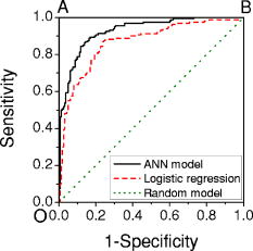 In a double-blinded test of the ANN, we fed the data from two new patients to evaluate its capability of predicting new results, the so-called generalization. The test set, described earlier in Sec. 2.2, comprised the Raman spectra of 40 cancerous and 40 normal cells. The network predicted correctly 17 of 20 cancer cells and 17 of 20 normal cells for the first patient and 17 of 20 cancer cells and 20 of 20 normal cells for the second patient. The overall sensitivity and specificity were 85% and 92.5% respectively, compared with the corresponding 82.5% and 92.5% of logistic regression. The limited improvement in the test may be due to the samples. In fact, the tissue specimens of the test set were graded as well-differentiated by pathology, and a higher degree of differentiation in pathology points to a smaller difference between the normal and abnormal. In pathological terms, well-differentiated tissues show a regular order similar to that of normal tissues, where there are clear structures. Also cells from well-differentiated tissues exhibit morphology similar to those in normal tissues, such as the cell shapes, nuclear sizes, and uniformity of cells inside the tissues. On the other hand, in poorly differentiated tissues, the cells are aligned in a chaotic way, indicating a higher degree of invasiveness. Here, our test results may provide evidence that morphological similarities and biochemical similarities between the well-differentiated cells and the normal cells are correlated. Nevertheless, the generalization of our ANN is excellent. A common problem in ANN algorithms is that a well-trained network predicts very poorly on new data. This is absent in our model. 3.2.Sensitivity AnalysisThe sensitivity map is presented in Fig. 4 . The split-half resampling technique was applied to investigate the reproducibility of sensitivity maps.16 The scores of 100 split-half resamplings (corresponding to 100 pairs of independent networks trained separately on split-half data) were found to be above 2.3657, corresponding to a minimum 99.1% confidence interval. Therefore, Fig. 4 is reproducible at above 99.1% confidence level. Fig. 4Sensitivity map of the network and the training data. Major features are identified here and listed in Table 2. Do not confuse the sensitivity here with that in Fig. 3.  Table 2Tentative assignments of the Raman bands identified in Fig. 4, mean intensity changes (increase + /decrease − ) of cancer relative to normal, and p-values of Student’s t-tests on band intensities. The spectral resolution of our system is 8cm−1 .
Prominent Raman bands are easily identifiable on Fig. 4. Tentative assignments23 are listed in Table 2 . Intensities at these peaks were read out from the data and subjected to Student’s t-test. We observed mean intensity increases from normal to cancer at 940.988, 1004, 1096.433, 1209.015, 1265.006, 1304.081, 1341.605, 1437.853, 1520.245, 1655.304, and and decreases at the remaining peaks. The increases occur mostly at the proteins and nucleic acids bands, indicating that cancer cells have higher DNA/RNA and protein activities. It is a surprise that glucose (decreasing, p- ) and cholesterol (increasing, p- ) appear on the list. However, signal alterations at 759.803, 940.988, 1004, 1096.433, 1209.015, 1341.605, and cannot be ruled out as statistical fluctuations (p- ). Furthermore, the cancer cells systematically (p- ) have lower signals than the normal ones in the spectral region below (see Fig. 1, for example), which may require further investigation. This phenomenon is also reflected in Fig. 4 as increased sensitivity levels at the same region, and confirmed by the colon tissue spectra in Fig. 5B of Ref. 23. Finally, even though mean intensity changes with p-values less than 0.05 are considered as statistically significant by medical doctors, a p-value greater than 0.05 does not necessarily reject the correlation of a band to the disease transformation. 3.3.Conclusions and DiscussionsIn this paper, we compared the technical characteristics of DNA FCM and LTRS, including working principles, sample preparations, hardware aspects, data collection schemes, operational procedures, and sample amount requirements, for single-cell investigation of cancers. LTRS can share the single-cell processing procedures already existing in hospitals for FCM, but removes the requirement of fluorescent dye staining. Unlike DNA FCM, which replies on the accumulative histogram of tens of thousands of cells, LTRS can decide on each individual cell, which makes LTRS very advantageous for diagnosing small tumors. In the meantime, by detecting the biochemical activities of cancers at the single-cell level, LTRS can provide deeper insight into the dynamics of carcinogenesis than tissue Raman spectroscopy, because cell functions are more fundamental than tissue functions. Potentially, single-cell LTRS can achieve higher accuracy than tissue Raman spectroscopy, because the course of carcinogenesis starts within the epithelial cells, and the epithelial cells are the primary source of diagnostic information for early cancer detection. In literature, some tissue components like collagen are reported to show correlations to cancer developments. However, because genetical alterations are the foundation of structural changes, variations in these components are by-products of carcinogenic activities in the epithelial cells and thus serve only as the secondary source of diagnostic information. Furthermore, many other tissue components do not possess diagnostic information at all. Tissue Raman spectroscopy suffers from two sources of interference: one is the Raman signal from the irrelevant tissue components; the other is the strong fluorescence and its associated noise from the tissue bulk. Even at 785-nm excitation, tissue fluorescence is still considerably higher than tissue Raman signal, and mathematical preprocessing such as fifth-order polynomial fitting is typically required to subtract the slow-varying fluorescence background from the data. Unfortunately, the noises associated with the fluorescence are left in the processed data. Therefore, in Raman studies, it is desirable to avoid as many fluorescence sources as possible. In a clinical study of colorectal adenocarcinoma, we measured the Raman spectra of 400 living epithelial cells from ten patients using LTRS. An ANN algorithm incorporating outlier probability corrections was developed to overcome the limitations existing in a previous study employing logistic regression.1 Remarkable improvements were achieved in the sensitivity and specificity of the predictions. Unavailable to logistic regression, the sensitivity map of ANN was evaluated to objectively quantify the contribution of each Raman frequency in the course of carcinogenesis. Important Raman bands were identified from the map, and Student’s t-tests were performed on their intensities. Unlike the subjective visual inspections commonly used in spectral analysis, the sensitivity map technique provides an objective, quantitative, and automatic way to discover important Raman peaks. In our experiments, only living epithelial cells were measured. The following discussions are restricted to living cells only. We cannot rule out the possibility of potential damage to some membrane proteins on the cell surface during the process of cell isolation from the tissue, but the primary culture procedure we employed is well-established and should reduce such damage to a minimum. In the meantime, the intracellular substances should be intact. Over the past decades, there have been intense studies on cancer cell culture techniques to prevent damage to the cells. Today, these techniques are already mature and widely applied in various fields. One example is the cell lines on the market, which came from the primary cultures originally harvested from patients. The demand for membrane protein protection might originally come from conventional FCM, which requires the binding of fluorescence markers to specific targets on the cell surface. After years of development, different protocols for different tissue types are already available in standard textbooks. LTRS on single cells can directly enjoy the fruits of other fields to keep possible cell damage under control. Furthermore, the major signal of LTRS originates from the volume inside the cell, so we do not expect a detectable alteration of the cell’s Raman spectrum due to the isolation processing. The average Raman spectra of single epithelial cells [Figs. 1a and 1b] share many common features with those of tissues (Fig. 5B in Ref. 23). They exhibit a general resemblance in the overall spectral shapes. However, differences in spectral details are obvious due to the extra components in tissue other than the epithelial cells. The difference spectra between the abnormal and the normal [Fig. 1c in this paper and Fig. 6B in Ref. 23] also show similarity in general trends, but differ in details. To establish our diagnostic model, we employed the tissue histopathology assessments as the golden standard and involved only those cases with consensus reached between two independent pathologists. A cell’s classification was set to the pathology classification of the tissue where it originated. There was a small possibility that a cell from a malignant tumor might be actually normal, resulting in an outlier. Unfortunately, it is impractical to obtain a cell’s classification from a direct single-cell histochemical analysis. To the best of our knowledge, immuno-histochemical analysis on cells/tissues is not for diagnostic purpose and cannot determine the normal/malignant nature of samples. It is rather used to supply assistive information for histopathology assessments. Besides, immuno-histochemical information alone is not reliable for diagnosis because the targeted proteins are also expressed in normal cells/tissues. Our way to assign a cell’s classification should provide the best accuracy for model training. In both the training set and the test set, around 14% of all cancer cells were misidentified by our model. But in our opinion, the outliers are only a minor source for this error, since it is highly unlikely that our cancer tissue samples contained such a high percentage of normal cells. As a matter of fact, our diagnostic model was built purely on experimental data with no prior knowledge and could be affected by the noises in the signals as well as the statistical nature of the individual variations of the cells. Unlike the training stage of our model, the application stage does not require prior histopathology assessment on a sample. LTRS diagnosis can be run independent of or without histopathology. In a clinical application, cells from suspected tumor sites can be retrieved through fine needle aspiration or exfoliative cytology methods like brushing and washing and then examined by LTRS to determine the nature of the cells. Frequently, doctors do not know the definitive characteristics of a suspected site without resorting to sophisticated diagnostic techniques. This is where histopathology, LTRS, DNA FCM, etc. come into play. In many situations, doctors need to know only whether a suspected cancer transform has occurred in the first place, before further investigation can be triggered to find its exact location. Exfoliative cells in pleural fluid, ascites, and urine can be collected and analyzed by LTRS to help doctors make decisions. The extension of our work to other epithelial cancers is straightforward. The single-cell diagnosis technique presented here can be directly applied to clinical tests. Thanks to FCM, preparation of single-cell suspensions is already routine in hospitals today. Further, exfoliative cytology can also provide samples to our technique. The low requirement for sample amounts makes our technique very attractive to cancer screening. The current work deals only with the question “Normal or cancer?” Future studies will focus on the subclassification of different tumor stages. AcknowledgmentsWe thank Dr. Sigurdsson for a private communication on artificial neural networks. This work was partially supported by Shanghai Optical-Tech Special Project Grant No. 036105016. ReferencesK. Chen,
Y. J. Qin,
F. Zheng,
M. H. Sun, and
D. R. Shi,
“Diagnosis of colorectal cancer using Raman spectroscopy of laser-trapped single living epithelial cells,”
Opt. Lett., 31 2015
–2017
(2006). https://doi.org/10.1364/OL.31.002015 0146-9592 Google Scholar
J. W. Chan,
D. S. Taylor,
T. Zwerdling,
S. M. Lane,
K. Ihara, and
T. Huser,
“Micro-Raman spectroscopy detects individual neoplastic and normal hematopoietic cells,”
Biophys. J., 90 648
–656
(2006). https://doi.org/10.1529/biophysj.105.066761 0006-3495 Google Scholar
K. G. MacLeod and
S. P. Langdon,
“Essential techniques of cancer cell culture,”
Methods Mol. Med., 88 17
–29
(2004). 1543-1894 Google Scholar
J. Costa and
C. Cordon-Cardo,
“Cancer diagnosis: molecular pathology,”
641
–657
(2001) Google Scholar
Australasian Flow Cytometry Group,
“Recommended guideline standards for DNA investigations,”
Purdue Cytometry CD-ROM, Purdue University, West Lafayette, IN (1997). Google Scholar
A. S. Haka,
K. E. Shafer-Peltier,
M. Fitzmaurice,
J. Crowe,
R. R. Dasari, and
M. S. Feld,
“Diagnosing breast cancer by using Raman spectroscopy,”
Proc. Natl. Acad. Sci. U.S.A., 102 12371
–12376
(2005). https://doi.org/10.1073/pnas.0501390102 0027-8424 Google Scholar
A. S. Haka,
K. E. Shafer-Peltier,
M. Fitzmaurice,
J. Crowe,
R. R. Dasari, and
M. S. Feld,
“Identifying microcalcifications in benign and malignant breast lesions by probing differences in their chemical composition using Raman spectroscopy,”
Cancer Res., 62 5375
–5380
(2002). 0008-5472 Google Scholar
P. Crow,
A. Molckovsky,
N. Stone,
J. Uff,
B. Wilson, and
L. M. Wongkeesong,
“Assessment of fiberoptic near-infrared Raman spectroscopy for diagnosis of bladder and prostate cancer,”
Urology, 65 1126
–1130
(2005). https://doi.org/10.1016/j.urology.2004.12.058 0090-4295 Google Scholar
M. Gniadecka,
P. A. Philipsen,
S. Sigurdsson,
S. Wessel,
O. F. Nielsen,
D. H. Christensen,
J. Hercogova,
K. Rossen,
H. K. Thomsen,
R. Gniadecki,
L. K. Hansen, and
H. C. Wulf,
“Melanoma diagnosis by Raman spectroscopy and neural networks: structure alterations in proteins and lipids in intact cancer tissue,”
J. Invest. Dermatol., 122 443
–449
(2004). https://doi.org/10.1046/j.0022-202X.2004.22208.x 0022-202X Google Scholar
J. T. Motz,
M. Fitzmaurice,
A. Miller,
S. J. Gandhi,
A. S. Haka,
L. H. Galindo,
R. R. Dasari,
J. R. Kramer, and
M. S. Feld,
“In vivo Raman spectral pathology of human atherosclerosis and vulnerable plaque,”
J. Biomed. Opt., 11 021003
(2006). https://doi.org/10.1117/1.2190967 1083-3668 Google Scholar
E. B. Hanlon,
R. Manoharan,
T. W. Koo,
K. E. Shafer,
J. T. Motz,
M. Fitzmaurice,
J. R. Kramer,
I. Itzkan,
R. R. Dasari, and
M. S. Feld,
“Prospects for in vivo Raman spectroscopy,”
Phys. Med. Biol., 45 R1
–R59
(2000). https://doi.org/10.1088/0031-9155/45/2/201 0031-9155 Google Scholar
Z. J. Smith and
A. J. Berger,
“Surface-sensitive polarized Raman spectroscopy of biological tissue,”
Opt. Lett., 30 1363
–1365
(2005). https://doi.org/10.1364/OL.30.003365 0146-9592 Google Scholar
G. P. Singh,
G. Volpe,
C. M. Creely,
H. Grotsch,
I. M. Geli, and
D. Petrov,
“The lag phase and G(1) phase of a single yeast cell monitored by Raman microspectroscopy,”
J. Raman Spectrosc., 37 858
–864
(2006). https://doi.org/10.1002/jrs.1520 0377-0486 Google Scholar
C. Xie,
J. Mace,
M. A. Dinno,
Y. Q. Li,
W. Tang,
R. J. Newton, and
P. J. Gemperline,
“Identification of single bacterial cells in aqueous solution using conflocal laser tweezers Raman spectroscopy,”
Anal. Chem., 77 4390
–4397
(2005). https://doi.org/10.1021/ac0504971 0003-2700 Google Scholar
K. W. Short,
S. Carpenter,
J. P. Freyer, and
J. R. Mourant,
“Raman spectroscopy detects biochemical changes due to proliferation in mammalian cell cultures,”
Biophys. J., 88 4274
–4288
(2005). https://doi.org/10.1529/biophysj.103.038604 0006-3495 Google Scholar
S. Sigurdsson,
P. A. Philipsen,
L. K. Hansen,
J. Larsen,
M. Gniadecka, and
H. C. Wulf,
“Detection of skin cancer by classification of Raman spectra,”
IEEE Trans. Biomed. Eng., 51 1784
–1793
(2004). https://doi.org/10.1109/TBME.2004.831538 0018-9294 Google Scholar
J. L. Deng,
Q. Wei,
M. H. Zhang,
Y. Z. Wang, and
Y. Q. Li,
“Study of the effect of alcohol on single human red blood cells using near-infrared laser tweezers Raman spectroscopy,”
J. Raman Spectrosc., 36 257
–261
(2005). https://doi.org/10.1002/jrs.1301 0377-0486 Google Scholar
G. Deinum,
D. Rodriguez,
T. J. Romer,
M. Fitzmaurice,
J. R. Kramer, and
M. S. Feld,
“Histological classification of Raman spectra of human coronary artery atherosclerosis using principal component analysis,”
Appl. Spectrosc., 53 938
–942
(1999). https://doi.org/10.1366/0003702991947829 0003-7028 Google Scholar
H. Nielsen,
“UCMINF—an algorithm for unconstrained nonlinear optimization,”
(2000). Google Scholar
D. J. C. MacKay,
“A practical Bayesian framework for backpropagation networks,”
Neural Comput., 4 448
–472
(1992). 0899-7667 Google Scholar
D. J. C. MacKay,
“The evidence framework applied to classification networks,”
Neural Comput., 4 720
–736
(1992). 0899-7667 Google Scholar
D. J. C. MacKay,
“Comparison of approximate methods for handling hyperparameters,”
Neural Comput., 11 1035
–1068
(1999). https://doi.org/10.1162/089976699300016331 0899-7667 Google Scholar
N. Stone,
C. Kendall,
J. Smith,
P. Crow, and
H. Barr,
“Raman spectroscopy for identification of epithelial cancers,”
Faraday Discuss., 126 141
–157
(2004). https://doi.org/10.1039/b304992b 0301-7249 Google Scholar
|
||||||||||||||||||||||||||||||||||||||||||||||||||||||||||||||||||||||||||||||||||||||||||||||||||||||||||||||||||||||||||||||||||||||||||||||||||||||||||||||||