|
|
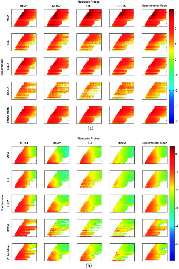
1.IntroductionFluorescence spectroscopy has the potential to provide real-time diagnosis of intra epithelial neoplasia; early clinical trials have shown increased specificity compared to white light endoscopy in a variety of clinical applications.1 For these technologies to be used routinely in the clinic, robust techniques to properly calibrate resulting spectra are required.2 Large multicenter clinical trials of this technology will require that data acquired from different spectrometers and fiber optic probes be combined for analysis with a single diagnostic algorithm. For example, we are testing fluorescence spectroscopy for detection of cervical neoplasia in screening and diagnostic populations. As part of the analysis presented here, we have acquired data with three different spectrometers and four fiber optic probes for interdevice verification. Existing literature is sparse with respect to prospective cross-validation or interdevice comparative studies of multiple medical instruments performed prior to clinical trials. In a study of confocal spectral imaging systems, Zucker and Lerner3 used a light source with an “absolute standard reference spectrum” on 10 systems that were yielding varying spectra. Through the use of the optical standard, they were able to make objective comparisons of the devices. Guo 4 utilized phantoms and analysis via analysis of variance (ANOVA) to determine the inter- and intradevice variability of dual energy x-ray absorptiometry (DXA) and found that the reliability of DXA devices was unpredictable. Using a potentially variable “standard,” Friedman 5 conducted a multicenter trial using five normal human subjects at nine different clinical sites to evaluate the interdevice differences in functional magnetic resonance imaging (fMRI) results. Finally, a study6 was conducted at 10 centers to determine the variability of 12 MRI systems using phantoms. This trial was unique in that it investigated the variability in short-term, daily, and midterm intervals to determine the frequencies required to conduct a quality control program. In this paper, we explore differences in data acquired with different spectrometers and fiber optic probes using optical calibration and verification standards2 over the course of a day for . Studies such as these are critical in understanding the variability between instruments when used in a multicenter trial. We previously conducted a study described in Lee 7 that analyzed raw, uncorrected spectroscopy data from different spectrometers and fiber optic probes. Here, we analyze data that have been calibrated in a method designed to remove variations due to the wavelength-dependent response of the fiber optic probes and intensity disparity of the spectrometers. Remaining variability within the processed data provides a better understanding of the technical limits of clinical application of fluorescence spectroscopy. This study assessed the repeatability of measurements across devices and within the same device across time. We further analyzed how each spectrometer performed with each of four fiber optic probes measuring three sets of 13 optical calibration standards. We repeated the measurements of one spectrometer to evaluate the effect of operator experience in performing the experiment. Additionally, because we believed that there may be variation from day to day and variation within a day, e.g., from warm-up, we measured three times per day for each of . Therefore, we designed a study to assess each of these six factors (spectrometer, fiber optic probe, optical calibration standards, measurement day, and measurement number within the day or time of day, and operator experience). Measurements were made at all combinations of these six factors. Unlike the study cited by Lee using uncorrected raw data, which used only the raw data, which is defined here as background subtraction, wavelength calibration, and integration time correction, we present the raw and fully processed data. 2.Materials and Methods2.1.Study DesignFigure 1 shows a schematic of the study design. As indicated in the figure, there were three spectrometers, labeled FEEM̱3(1), FEEM̱3(2), FEEM̱3(3), referred to as spectrometers MDA, LBJ, and BCCA, respectively. Each of the spectrometers is in a different location: FEEM̱3(1) is located at the Colposcopy Clinic of the University of Texas M. D. Anderson Cancer Center in Houston, Texas (MDA); FEEM̱3(2) is located at the Lyndon B. Johnson (LBJ) County Hospital in Houston, Texas; and FEEM̱3(3) is located at the Colposcopy Clinic of British Columbia Cancer Agency in Vancouver, British Columbia, Canada (BCCA). The spectrometers are difficult to move, so we left them in their respective locations and brought all other materials to them. Each spectrometer has a standards tray, which contains 13 optical standards, which were shipped between sites for this study. The fiber optic probes were generally attached to particular spectrometers, but we shipped them between sites as well. Every fiber optic probe, standards tray, and the calibration standards themselves were labeled prior to conducting the study. The study was designed by the statisticians and principal investigator (DC, MF). The study involved the three spectrometers, four fiber optic probes, and three sets of optical calibration standards. There were a total of 4 (measurements within each day) = 288 measurements made on each of the 13 individual optical calibration standards. Measurements were made by one research assistant (OS) in the dark, assisted by a senior clinical biomedical engineer (RP). The data, consisting of approximately , was quality assured by the codirector of the instrumentation core (BP) and the senior programmer (DS). The first analysis reported by Lee involved the raw data. The subsequent analyses reported here were carried out by the codirector of the instrumentation core, the programmer, and the director of the biostatical core and the research assistant (BP, DS, DC, and OS). The ramifications of the analysis were discussed with the codirector of the instrumentation core (NMcK) and other members of the instrumentation team (CMacA and RRK). 2.2.Use of Spectroscopic MeasurementsFluorescence spectroscopy involves illuminating the tissue sample with excitation light and measuring the emitted light at longer wavelengths. Our devices use light delivered through a fiber optic probe that also collects the light that is fluoresced. The data are stored as an intensity at each excitation-emission wavelength. The fluorescence in tissue comes from several biologically relevant fluorophores including NADH, FAD, tryptophan, elastin, and collagen. Absorbers, such as hemoglobin, also contribute to tissue fluorescence by absorbing excitation light and remitted fluorescence. There has been some success using fluorescence spectroscopy to detect cancer and precancer.8, 9, 10, 11, 12 An important issue in the successful implementation of any optical device is calibration of the spectroscopic system and control of extraneous factors. Control of these factors in spectroscopy depends on the timely measurements of standards. In the following sections, we describe the optical instrumentation and calibration standards used to control and study these factors. 2.3.Spectroscopic InstrumentationThe fast excitation emission matrix (FastEEM) systems are spectroscopic devices for measuring the intensity of fluorescence at a variety of excitation and emission wavelengths. Typically, the excitation light is conducted through a fiber optic cable to a probe to illuminate the sample. The fiber optic probe itself is fairly small (diameter ). At the distal tip of the fiber optic probe, a mixing element that consists of a large diameter optical fiber uniformly illuminates the sample with the excitation light and collects the emitted light from the same area. The emission light is then conducted through another set of fibers in the probe back to a diffraction grating, which separates the wavelengths and projects the emitted light onto a charge-coupled device (CCD). There are a number of components of such a system which can vary under temperature, age, and other factors, thus requiring highly precise calibration by measuring standards with known optical response. Figure 2 shows a block diagram of the FastEEM3 spectrometer. Broadband illumination is provided by a xenon arc lamp, and a set of filters selects the desired part of the excitation spectrum. Fluorescence is measured at excitation wavelengths from in increments of , with a FWHM of . Fig. 2Schematic of fast-EEM3. Xe LS, xenon light source; , fluorescence excitation filter wheels; , TS, translation stage; P2, sampling powermeter; P1, probe powermeter; T, tungsten light source; M, mercury-argon light source; IS, integrating sphere; , fluorescence emission filter wheel; Spx, spectrometer. 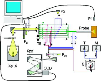 The exterior of the fiber optic probes for FastEEM3 are stainless steel, long, and houses 24 excitation and 12 collection fibers. Probes were tipped with a quartz mixing element in diameter with a length of which enables roughly uniform illumination of the portion of the sample queried and collection from the same area. We used four probes throughout the course of the study. The four probes were made by three different manufacturers: Multimode (Richmond, Virginia), PNP Optica (Kitchener, Ontario), and Ceramoptec (East Longmeadow, Massachusetts). 2.4.Standards Measured in the StudyStandards for the calibration of fluorescence include rhodamine (peak emission wavelength at ), exalite (peak emission wavelengths at 370 and ), and coumarin (peak emission wavelength at ) as positive standards, and deionized water and a frosted quartz cuvette as negative standards. Three different calibration light sources include a mercury-argon lamp, a deuterium-halogen lamp, and a tungsten lamp to calibrate the wavelength and spectral sensitivity. A National Institute of Standards and Technology (NIST)-traceable tungsten light source is used to determine the spectral sensitivity of the spectrometer. The optical transfer function is calculated and applied to the tissue spectral during the calibration process (step 4 in the following). In this paper, we analyze the results from the positive standard rhodamine ( solution of rhodamine 610 dissolved in ethylene glycol) and the negative standards, frosted quartz cuvette and water. Results from the positive standards, coumarin and exalite, are similar to those of rhodamine and are not presented here. The data were processed using the method described in Ref. 2. The process consists of (1) calibrating the wavelength using the mercury-argon lamp, with an additional wavelength offset correction from the rhodamine peak position, taken from the closest (in time) rhodamine measurement; (2) subtracting the background; (3) dividing the fluorescence intensity by the excitation power meter measurement and exposure time; (4) correcting for the nonuniform spectral response of the fiber optic probe and spectrometer; and (5) normalization by the intensity of rhodamine at an excitation of and an emission of . Data were smoothed as is done for tissue measurements. Data processing was done with code written in MATLAB (Natick, Massachusetts). 2.5.Trial Design for Standards MeasurementsWe took measurements using each of the three FastEEM spectrometers for every possible combination of three calibration standards trays and four fiber optic probes. Measurements were made over for each spectrometer and fiber optic probe combination. The different standards trays were rotated three times in each day because it was unknown whether the variations of the xenon lamp, spectrometer heating, inconsistent contact between the fiber optic probe and standard, or other unknown sources introduced variability within a day or from day to day. Thus, there were a total of 288 measurements made on each of the thirteen individual standards. Additionally, the measurements on the LBJ spectrometer were repeated at the end of the study. One research assistant made all the measurements. The measurements were obtained in the same order when interchanging the standards trays. Every measurement was timed and recorded into a log file along with detailed descriptions of any problems which were encountered. The problems were discussed daily with members of the instrumentation core. 2.6.Statistical MethodsThe statistical analysis was based on ANOVA, including multivariate ANOVA (MANOVA) and enabled us to quantify the contribution of each factor (and higher order interactions of two or more factors) in terms of the proportion of variance explained and the statistical significance of the factor as a source of variation. All statistical analyses were performed in MATLAB or R (available for free from Ref. 13). The first objective was to perform a MANOVA including the main effects from all factors. However, since the data are hyper-dimensional (each observation has over 4000 intensity values at the different excitation-emission wavelength combinations), one cannot perform a MANOVA on the raw data as the estimated covariance matrix will be singular.14, 15 To eliminate this problem, we first performed a principal components analysis (PCA) of the processed data for each optical standard taken during the study and selected enough principal components to capture 99% of the variability so that the principal component data is an accurate approximation of the original data. This reduced the data sufficiently that MANOVA could be performed. Any factors that were found significant were kept for a second stage of the analysis wherein we performed ANOVA on each of the principal component scores to find the percentage of variability explained by each of the significant factors. Then, we computed an overall percentage of variance explained for each significant factor as a weighted average of the percentage of variance explained across the principal components using as weights the percentage of variance corresponding to the principal component. 3.Results3.1.Initial Data AnalysisThe variations among spectrometers and optical probes were plotted for both raw and processed data. Figures 3, 4, 5 show the mean raw and processed EEMs of rhodamine, frosted cuvette, and water organized by spectrometer and fiber optic probe. The overall mean is in the right lower plot. Figure 3 shows raw and processed EEMs of rhodamine; excitation wavelengths along the ordinate, emission wavelength along the abscissa, and the of the fluorescent intensities are represented with a MATLAB “jet” color map. Fig. 3(a) Raw and (b) processed data of the standard rhodamine, a positive standard. EEM plot matrices of the probe study plotted on a log scale. The vertical axis is the excitation wavelength ranging from (tick marks at intervals). The horizontal axis represents the emission wavelengths ranging from (tick marks at intervals). Each individual box-probe combination EEM is the mean of six measurements: three measurements per day for . The first four columns represent the results from the probes, while the first four rows represent the four box measurements. The right lower quadrant is the overall mean of both types of equipment.  Fig. 5(a) Raw and (b) processed data of the standard frosted cuvette, a negative standard. EEM plot matrices are in the same arrangement as in Fig. 3.  The raw data, shown in Figs. 3a, 4a, 5a, demonstrate significant differences in the data. The most prominent differences of the raw data are (1) light source intensity of the spectrometers, (2) the transmission efficiency of the fiber optic probes, and (3) the “noisier” BCCA spectrometer. A source of the raw intensity differences when comparing the boxes is due to the illumination intensity of the xenon light source. All xenon bulbs were of the same model, but the intensity decreases with usage. Measurements demonstrated that the xenon light source intensity at BCCA and LBJ were at approximately 10 and 30% of the MDA box, respectively. The reduced raw intensity of the MDA1 and, to a lesser extent, the LBJ fiber optic probes are due to their reduced optical transmission despite the same specifications given to the various probe manufacturers. The transmission of the probes as compared to the BCCA probe are 26, 89, and 47% for the MDA1, MDA2, and LBJ probes, respectively, at . To compare the CCD noise of the three FastEEM3 spectrometers, data were recorded from each with all shutters closed to monitor the CCD dark current and readout noise. Although all three CCDs were within their noise specifications, marked differences in performance were evident. The mean counts per pixel of the BCCA, LBJ, and MDA CCDs are 445.23, 511.73, and 475.68, respectively. The coefficients of variation, which describe the variable noise, of the BCCA, LBJ, and MDA CCDs are 0.081, 0.095, and 0.057%, respectively. 3.2.Processed Data AnalysisProcessing the data, as shown in Fig. 3b, 4b, 5b, removes the majority of the differences in the xenon lamp and spectrally uniform probe attenuation. The variation of the data caused by lamp intensity and probe transmission after processing is dramatically reduced, but the marked differences of autofluorescence in the fiber optic probes then becomes the major source of variation. The processing step 4 (Sec. 2.4), which corrects for the nonuniform spectral response of the fiber optic probe and spectrometer is unable to account for the fiber optic probe autofluorescence. The MDA1 fiber optic probe has a marked autofluorescence compared to the other probes used in this study and is evident in the processed plots. Our group is investigating whether the fiber optic probe autofluorescence can be removed from the previously measured tissue spectroscopic measurements. Additionally, only the MDA1 fiber optic probe was used on an appreciable number of patients. The vast majority of patients were measured using the BCCA probe. Due to the variability among probes evidenced in this study, we isolated the problem and are now constructing the fiber optic probes in our lab for further clinical trials. We implemented a stringent quality control process in the manufacturing of the fiber optic probes. 3.3.ANOVA AnalysisThe ANOVA analysis was conducted on a dimensionally reduced data set obtained14 by PCA because the actual data have many more variables than observations. In every case, we selected enough principal components (PCs) to capture 99% of the variability. Table 1 shows the number of PCs required to explain 99% variance. For rhodamine, we see that one PC in the raw data captures at least 99% of the data. This component is essentially the shape of the rhodamine spectrum and the corresponding PC score is the amplitude. There are large amplitude variations between devices, but these are mostly removed by the processing and one sees that it requires 33 PCs to explain 99% of the variance in the fully processed rhodamine. The large number of components required indicates that the overall variability is less. Table 1The number of PCs required to explain 99% variance.
Once the dimensionalities of the data were sufficiently reduced we conducted a standard multivariate ANOVA using Wilk’s test statistic.14 Each factor was included only as a main effect in this analysis. The results are presented in Table 2 in which we examine the values. We see that with one exception, only the spectrometer and fiber optic probe are significant sources of variation. The one exception is that for fully processed rhodamine, the standards tray is a significant source of variation. In this case, the percentage variance explained is less than 1%. Thus, in general, most of the standards trays, day-to-day variation, and order of measurement are not statistically significant. For all factors, we further analyzed the percentage of variance explained, including all possible interactions, as shown in Table 3 . These results show that the processing reduces most of the variability due to these extraneous factors. For the frosted cuvette, the main effect due to the spectrometer accounts for 72% of the variance in raw data, but goes down to 1% in the fully processed data. Thus, the processing eliminates most of the effect due to the spectrometer alone. Similarly for the effect due to the spectrometer, the percent variance explained in water goes down 82% before processing to 0.5% after processing, and in rhodamine from 56 to 9%. The effect due to probe alone shows similar but less dramatic differences (11 to 6% for the frosted cuvette and 21 to 4% in rhodamine). The one case in which processing increases the variance explained is water where the fiber optic probe effect rises from 5 to 11%. The increased variance of the probe contribution is explained by the autofluorescence of the fiber optic probes. Note the dramatic decrease in percentage of variance explained for the spectrometer after processing, which is consistent with reducing the differences in lamp output of the spectrometers. With processing, this variation nearly disappears and the percent variance explained by the autofluorescent probe takes precedence with this negative standard. Table 2The P values from the MANOVA for optical standards on frosted cuvette, water, and rhodamine.
This statistical analysis also included interaction terms. For example, the spectrometer-fiber optic probe interaction term measures how much the mean for a particular spectrometer and fiber optic probe combination differs from the predicted value obtained by adding the mean for that spectrometer and the mean for that fiber optic probe. For all three standards, there was substantial reduction in this term following processing. In the case of fully processed rhodamine where the standards tray was significant, we have included all the interactions of this factor with spectrometer and fiber optic probe as well as the three-way interaction, which describes the output that can not be predicted from either the three individual components or one component and a two-way interaction. It is interesting to look at the rows of each type of measurement in Table 3. These rows sum to less than 100%, with the remainder being the unexplained variation (or “mean square due to error”). For instance, in raw rhodamine the row sum is 99%, indicating that almost all of the variability is due to the spectrometer, fiber optic probe, and their interaction. For fully processed rhodamine, the spectrometer alone accounts for 9% of the variance explained, the fiber optic probe for 4%, the standards tray for less than 1%, the spectrometer-fiber optic probe for 5%, the spectrometer-tray for 2%, the fiber optic probe-tray for 1%, and the spectrometer-fiber optic probe-tray for 5%. 3.4.Contrast PlotsFigure 6 presents contrast plots of the processed rhodamine. Contrast plots are used to emphasize the differences from the mean of the data set. The contrast plots of the spectrometer (or fiber optic probe) means are computed by subtracting the overall mean from the processed data of the spectrometer (or fiber optic probe) mean. The individual spectrometer-fiber optic probe combination contrast plots are computed by subtracting the corresponding spectrometer mean and fiber optic probe mean from the spectrometer-fiber optic probe combination mean and adding the overall mean. The contrast plots highlight the differences in the processed rhodamine at excitation wavelengths 300, 510, 520, and . The marked discrepancies at these excitation wavelengths led us to perform the statistical analysis using only excitation wavelengths and is termed “reduced EEM” in the tables. The reduced EEM of rhodamine decreases the variance explained from 9 to 4% for the spectrometer and is decreased to the level of the effect of the fiber optic probe. This analysis suggests that the data generated from excitation wavelengths 300, 510, 520, and with our current instrumentation are variable between spectrometers. At an excitation wavelength of we expect this to be due to the low intensity of rhodamine, but we are unsure of the cause at the higher excitation wavelengths. However, our algorithm does not use the aforementioned excluded excitation wavelengths in our current study of cervical neoplasia. Fig. 6Contrast plots of processed rhodamine in the same arrangement as Fig. 3. The white regions are where the comparisons ares nearly equal, while the gray area contain no EEM data. Note the marked differences in the extreme lower and upper excitation wavelengths.  Table 3Percentage of variance explained by each factor and their interactions for optical standards frosted cuvette, water, and rhodamine.
4.DiscussionDespite careful construction and standardization of design, differences remain among spectrometers including operator experience, fiber optic probes, their combination, and the rhodamine standard that are difficult to sort out. In these analyses, we learned that from the raw data, there were effects of spectrometers, fiber optic probes, and the spectrometer fiber optic probe interaction were of significance whereas time of day and day-to-day variation did not affect the data in a statistically significant manner. 16, 17, 18, 19, 20, 21, 22, 23, 24, 25 We further learn from the raw data that much of the variance can be explained by the spectrometer , the fiber optic probe , and their interaction . Rhodamine, a positive standard, accounted for 9% of variance even when the data were processed. However, the processed rhodamine variance in the spectrometer was decreased to the same variance as the fiber optic probe (4%) when using the reduced excitation spectra. Though the MANOVA analysis showed significant device effects, the figures for the raw data suggested that the device effects were largely the differences of the xenon light source, fiber optic throughput, and noise. A review of the processed data shows that the device effect was substantially reduced after processing. The noise of the BCCA device is evident in nonfluorescent portions of the EEM after processing. However, the SNR for tissue measurements in the BCCA spectrometer are , and thus we believe that the effects of noise are not significant is altering diagnostic performance.26 We will soon bring another optical device, three multispectral digital colposcopes (MDCs), to clinical trials at multiple sites. From the knowledge gained in our previous trials with the spectrometers and the study described here, we will implement a full factorial analysis prior to introduction in the clinic. Studies of device performance are rarely performed during clinical trials, yet add meaningful and confirmatory data about instrument performance. Clearly, device trials are important methodological issues for optical device trials and must be included in the quality assurance studies for the clinical trial design. We built a shorter but similar type of study into our quality control for these devices every . In the smaller partial factorial studies, we will measure and evaluate optical standards used for calibration of data. The methodology for studies such as the large study reported here are under development. Undoubtedly, an interdevice evaluation is critical for the conduct of clinical trials with multiple sites and devices to deconvolve the sources of variability in instrumentation which are assumed to be equivalent. ReferencesN. Ramanujam,
M. F. Mitchell,
A. Mahadevan,
S. Thomsen,
A. Malpica,
T. Wright,
E. N. Atkinson, and
R. Richards-Kortum,
“Spectroscopic diagnosis of cervical intraepithelial neoplasia (CIN) in vivo using laser-induced fluorescence spectra at multiple excitation wavelengths,”
Lasers Surg. Med., 19 63
–74
(1996). https://doi.org/10.1002/(SICI)1096-9101(1996)19:1<63::AID-LSM8>3.0.CO;2-O 0196-8092 Google Scholar
N. Marin,
N. McKinnon,
C. MacAulay,
S. K. Chang,
E. N. Atkinson,
D. D. Cox,
D. Serachitopol,
B. Pikkula,
M. Follen, and
R. Richards-Kortum,
“Calibration standards for multicenter clinical trials of fluorescence spectroscopy for in vivo diagnosis,”
J. Biomed. Opt., 11
(1), 024031
(2006). 1083-3668 Google Scholar
R. Zucker and
J. T. M. Lerner,
“Wavelength and alignment tests for confocal spectral imaging systems,”
Microsc. Res. Tech., 68 307
–319
(2005). 1059-910X Google Scholar
Y. Guo,
P. W. Franks,
T. Brookshire, and
P. A. Tataranni,
“The intra- and inter-instrument reliability of DXA based on ex vivo soft tissue measurements,”
Obes. Res., 12 1925
–1929
(2004). 1071-7323 Google Scholar
L. Friedman,
G. H. Glover,
D. Krenz, and
V. Magnottad,
“Reducing inter-scanner variability of activation in a multicenter fMRI study: role of smoothness equalization,”
Neuroimage, 32 1656
–1668
(2006). 1053-8119 Google Scholar
P. Colombo,
A. Baldassarri,
M. Del Corona,
L. Mascaro, and
S. Strocchi,
“Multicenter trial for the set-up of a MRI quality assurance programme. Magnetic Resonance Imaging,”
Magn. Reson. Imaging, 22 93
–101
(2004). 0730-725X Google Scholar
J. S. Lee,
O. Shuhatovich,
R. Price,
B. Pikkula,
M. Follen,
N. McKinnon,
C. MacAulay,
B. Knight,
R. Richards-Kortum, and
D. D. Cox,
“Design and preliminary analysis of a study to assess intra-device and inter-device variability of fluorescence spectroscopy instruments for detecting cervical neoplasia,”
Gynecol. Oncol., 99 S98
–111
(2005). 0090-8258 Google Scholar
T. J. Romer,
M. Fitzmaurice,
R. M. Cothren,
R. Richards-Kortum,
R. Petras,
M. V. Sivak Jr., J. R. Kramer Jr.,
“Laser-induced fluorescence microscopy of normal colon and dysplasia in colonic adenomas: implications fro spectroscopic diagnosis,”
Am. J. Gastroenterol., 90
(1), 81
–187
(1995). 0002-9270 Google Scholar
R. Richards-Kortum and
E. Sevick-Muraca,
“Quantitative optical spectroscopy for tissue diagnosis,”
Annu. Rev. Phys. Chem., 47 555
–606
(1996). https://doi.org/10.1146/annurev.physchem.47.1.555 0066-426X Google Scholar
N. Ramanujan,
M. F. Mitchell,
A. Mahadevan-Jansen,
S. L. Thomsen,
G. Staerkel,
A. Malpica,
T. Wright,
E. N. Atkinson, and
R. Richards-Kortum,
“Cervical precancer detection using a multi-variate statistical algorithm based on laser-induced fluorescence at multiple excitation wavelengths,”
Photochem. Photobiol., 64
(4), 720
–35
(1996). 0031-8655 Google Scholar
E. Svistum,
R. Alizadeh-Naderi,
A. El-Naggar,
R. Jacob,
A. Gillenwater, and
R. Richards-Kortum,
“Vision enhancement system for detection of oral cavity neoplasia based on autofluorescence,”
Head Neck, 26
(3), 205
–215
(2004). 1043-3074 Google Scholar
S. K. Chang,
Y. N. Mirabal,
E. N. Atkinson,
D. Cox,
A. Malpica,
M. Follen, and
R. Richards-Kortum,
“Combined reflectance and fluorescence spectroscopy for in vivo detection of cervical pre-cancer,”
J. Biomed. Opt., 10
(2), 24031
(2005). 1083-3668 Google Scholar
A. C. Rencher, Methods of Multivariate Analysis, 2nd ed.Wiley, New York
(2002). Google Scholar
A. Agresti, Categorical Data Analysis, 2nd ed.Wiley, New York
(2002). Google Scholar
K. A. Baggerly,
J. S. Morris,
S. Edmonson, and
K. A. Baggerly,
“Serum proteomics profiling—a young technology begins to mature,”
Nat. Biotechnol., 23
(3), 291
–292
(2005). 1087-0156 Google Scholar
K. A. Baggerly,
J. S. Morris, and
K. R. Coombes,
“Reproducability of SELDI-TOF protein patterns in serum: comparing datasets from different experiments,”
Bioinformatics, 20
(5), 777
–785
(2004). 1367-4803 Google Scholar
K. R. Hess,
W. Ahang,
K. A. Baggerly,
D. N. Stiver, and
K. R. Coombes,
“Microarrays: handling the deluge of data and extracting reliable information,”
Trends Biotechnol., 19
(11), 463
–468
(2001). 0167-7799 Google Scholar
K. R. Coombes,
W. E. Highsmith,
T. A. Krogmann,
K. A. Baggerly,
D. N. Stiver, and
L. V. Abruzzo,
“Identifying and quantifying sources of variation in microarray data using high density cDNA membrane arrays,”
J. Comput. Biol., 9
(4), 655
–669
(2002). 1066-5277 Google Scholar
L. Ramdas,
K. R. Coombes,
K. Baggerly,
L. Abruzzo,
W. E. Highsmith,
T. Krogmann,
S. R. Hamilton, and
W. Zhang,
“Sources of nonlinearity in cDNA microarray expression experiments,”
Genome Biol., 2
(11),
(2001). Google Scholar
K. R. Coombes,
S. Tsavachidis,
J. S. Morris,
K. A. Baggerly,
M. C. Hung, and
H. M. Kuerer,
“Improved peak detection and quantification of mass spectrometry data acquired from surface-enhanced laser desorption and ionization by denoising spectra with the undecimated discrete wavelet transform,”
http://www.mdanderson.org/pdf/biostats_utmdabtr-001-04.pdf Google Scholar
K. A. Baggerly,
J. S. Morris,
S. Edmonson, and
K. R. Coombes,
“Signal in noise: can experimental bias explain some results of serum proteomics tests for ovarian cancer?,”
J. Natl. Cancer Inst., 97
(6), 307
–309
(2005). 0027-8874 Google Scholar
M. Guillaud,
D. Cox,
K. Adler-Storthz,
A. Malpica,
G. Staerkel,
J. Matisic,
D. Van Niekerk,
N. Poulin,
M. Follen, and
C. MacAulay,
“Quantitative histopathological analysis of cervical intraepithelial neoplasia sections: methodological issues,”
Cell. Oncol., 26 31
–43
(2004). Google Scholar
D. Chiu,
M. Guillaud,
D. Cox,
M. Follen, and
C. MacAulay,
“Quality assurance system using statistical process control: an implementation for image cytometry,”
Cell. Oncol., 26 101
–17
(2004). Google Scholar
M. Follen,
S. Crain,
C. MacAulay,
K. Basen-Engquist,
S. B. Cantor,
D. Cox,
E. N. Atkinson,
N. MacKinnon,
M. Guillaud, and
R. Richards-Kortum,
“Optical technologies for cervical neoplasia: update of an NCI program project grant,”
Clin. Adv. Hematol. Oncol., 3 41
–53
(2005). Google Scholar
U. Utzinger,
E. V. Trujillo,
E. N. Atkinson,
M. F. Mitchell,
S. B. Cantor, and
R. Richards-Kortum,
“Performance estimation of diagnostic tests for cervical precancer based on fluorescence spectroscopy: effects of tissue type, sample size, population, and signal-to-noise ratio,”
IEEE Trans. Biomed. Eng., 46 1293
–1303
(1999). https://doi.org/10.1109/10.797989 0018-9294 Google Scholar
|