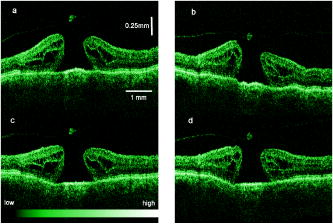
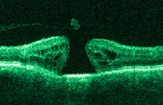
1.

Introduction

Optical coherence tomography (OCT) has become an important biomedical tissue imaging technique over the last decade.^{1, 2} Especially, it has proven very promising within the area of ophthalmology, where it is currently being applied both qualitatively and quantitatively for a large variety of diseases. As a result, third-generation commercial systems (third-generation time-domain) already are available for this application area. Ophthalmic OCT systems are beneficial both for diagnosing retinal diseases and also in obtaining novel knowledge about the retinal structure and the development of different pathologies.

Because OCT is based on low-coherence interferometry, the measured signals are affected by speckle noise,³ which can significantly lower the obtained signal-to-noise ratio (SNR) of the measured images. As the recorded speckle patterns will vary only in cases when the imaging geometry or setup is modified, either the position of the sample or the optical pathway should be allowed to vary between recorded scans to take advantage of repeated measurements in lowering the noise level. Frequency, spatial, angular compounding, and polarization diversity are possible ways^{3, 4} to decorrelate the speckle noise from one image to the next. If the speckle is fully uncorrelated between images, the SNR of the resulting average image is increased as the square root of the number of images used.⁵ For standard OCT commercial systems, such modifications of the measuring setup are not an option, and one is then left with the possibility of denoising the images using image post-processing techniques.^{6, 7} A simple approach is to apply a median filter or different kinds of low-pass filtering. More advanced schemes use adaptive wavelet schemes combined with nonlinear thresholds.⁸ Nonlinear anisotropic filtering has recently been suggested for enhancing retinal OCT images, and it was reported to facilitate segmentation of the retinal layers.⁹ One problem with these more advanced post-processing techniques is that there is a risk of generating artificial structures from the noise when applying the filters. We have found this to be a potential problem when doing image post-processing based on, e.g., coherent enhancing diffusion filters.¹⁰ Such problems are avoided if one instead implements an average procedure that calculates the statistical mean of the signal over different realizations of the stochastic process responsible for the noise.

When applying OCT for in vivo imaging of the human retina, small movements of the head and saccadic eye movements will lead to small axial movements of the retina relative to the imaging geometry during image recording. This behavior will in reality lead to decorrelation of the speckle noise from one image to the next when recording a series of B-scans. The challenge, under the assumption that mesoscopic landmarks can be correlated, is to register these and shift and distort the consecutive tomograms for successful averaging.

This paper illustrates how the disturbing noise including speckle can be significantly suppressed by combining a series of recorded OCT images, typically 8 to 12. The algorithm fuses a technique for aligning a series of one-dimensional (1-D) signals with a regularized dynamic programming algorithm that takes into account the spatial constraints/relationships of the two-dimensional images (i.e., using the fact that the estimated registration shift of a given A-scan should be correlated with the expected registration shifts of the neighboring A-scans). The resulting improvement facilitates quantification and clinical interpretation and has already proven most helpful for a number of pathologic applications. Initial reports on contrast enhancement of ophthalmic OCT images from combination of B-scans (using a less-rigorous and a less-robust approach than the methodology presented here) was reported in Ref. 11.

In Sec. 2, the image registering problem is formulated. Next, in Secs. 3, 4, 5, 6, the algorithmic approach based on regularized dynamic programming is outlined and illustrated for a specific case. In Sec. 7, the resulting improvement in image quality is both illustrated visually and quantified using a suitable contrast to noise measure. The clinical value of the image enhancement is illustrated from a number of cases in Sec. 8. The paper concludes with a discussion in Sec. 9. OCT is today a standard imaging technique in ophthalmological clinics focusing on retinal diseases. Accordingly, the results of applying the suggested method were based on a retrospective analysis of digital image information and did not require institutional review.

2.

Setup and Problem Formulation

The OCT data was recorded at Glostrup Hospital in Copenhagen using the Stratus/OCT3 instrument (Humphrey-Zeiss). The Stratus system provides as a standard 512 A-scans per B-scan, independent of the length of the physical scan length. The optical transverse resolution is $20\mu \mathrm{m}$ , and the axial resolution is approximately $10\mu \mathrm{m}$ . Accordingly, a standard $6\text{-}\mathrm{mm}$ -long scan has a lateral pixel spacing below the transverse resolution of the optical system.

Figure 1a shows a series of successive retinal B-scans corresponding to the ideal scan path illustrated in the autofluorescence fundus photograph [Fig. 1b]. It is clearly observed how small changes in eye position relative to the imaging device result in axial displacements of the retinal structure. Our goal is to enhance the SNR by registering such a series of images in order to calculate an average B-scan image.

Fig. 1

(a) B-scan measurements from the ideal scan path illustrated in the autofluorescence fundus photograph in (b) (line not to scale—width/length). Observe the axial shifts between corresponding A-scans.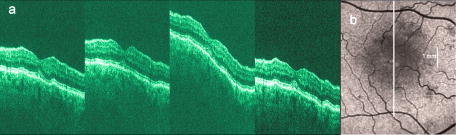

In order to fuse the individual B-scans into a single average image, we need to register the images mutually. Corresponding A-scans (represented by image columns) must be registered vertically to deal with the axial displacements. As we want to ensure a noise-robust registration procedure, we will use a so-called regularized algorithm, which takes the spatial continuity of the retinal structure into account.

In addition to the axial displacements, the inevitable eye movements will cause the sampled scanning points to scatter around the desired scan path. These movements include micro-saccade and tremor, which goes up to $15\mathrm{Hz}$ of rapid involuntary random motion in transverse and torsional directions. Large transverse shifts are more likely to happen if the patient has difficulties in fixating on the spot of the guiding beam used during recording of a B-scan. The transverse uncertainty naturally relates to the severity of the pathology of the retina being examined.

Part of the transverse displacements can be dealt with by combining the vertical registrations (corresponding to axial registration) with a possible rigid horizontal registration of one image to another, i.e., all rows in an image must be shifted the same amount relative to one of the other images to maximize an adequate similarity measure. Even though the horizontal registration can significantly reduce the effect of transverse distortions, the fact that the loci of the A-scans scatter around the ideal scan path will naturally lead to some loss of transverse resolution in the combined average image compared to that of a singe B-scan. In Sec. 6, we estimate the transverse accuracy that can typically be obtained when producing an average image with increased SNR. The process of registering two OCT images will be illustrated with the two images shown in Figs. 2a and 2b .

Fig. 2

(a) and (b) Two OCT images from the same retinal location. The scan length is $6\mathrm{mm}$ . (c) and (d) Mutually aligned versions of (a) and (b), respectively.

3.

Alignment Procedure

When axially registering the two B-scans in Figs. 2a and 2b, the objective is to find the vertical shifts between corresponding columns that will align them optimally according to a similarity measure. Here we apply the cross-correlation between shifted versions of image columns to measure how well they align. Because of the speckle noise (as well as other noise contributants), the shift leading to the maximum correlation does not necessarily specify the optimum position for an ideal alignment. We can, however, take advantage of the fact that axial shifts across the image in most cases is known to change smoothly and continuously, simply because the head/eye movements that have caused these shifts describe a continuous and smooth motion. (If a saccade or blink completely obscures the continuity of a B-scan, it is simply discarded by the user; see Sec. 9). The implication is that the obtained values of neigboring translation shifts (obtained by mutually registering two B-scans) must describe a continous and smooth curve. Such a constraint can be implemented using so-called regularization in combination with a dynamic programming algorithm.¹² In our case, this is analogous to formulating a constrained shortest-path strategy for navigating through an energy landscape specifying the problem at hand. The regularization then corresponds to applying a penalty term, adding extra cost to the traversed path through the landscape. The penalty will be dependent on the curvature and smoothness of the path. More precisely, we apply a regularized shortest path (or regularized minimum cost) algorithm to an image map or energy landscape $E(n,j)$ formed by calculating the negative cross-correlation for the possible vertical shifts ( $n$ -variable) between corresponding columns ( $j$ -variable) in the two considered B-scan images $I_a$ and $I_b$ (each with $N$ rows and $M$ columns):

4.

Regularized Dynamic Programming

Dynamic programming describes a methodology where optimal solutions of subproblems can be used to find the optimal solutions of the overall problem. A well-known application is to determine the shortest path or accumulated cost across a map/image. Its general principles were first introduced by Bellman.¹³ Dynamic programming is known to be computationally efficient and to find the optimal path, but in its original version, it does not allow for any smoothness constraints on the generated path across the image. An extension was introduced in Ref. 14, which applied a penalty depending on the shape of the contour. To maintain optimality, it was an iterative process. The method was adapted by Buckley in Ref. 12, where a method for finding smooth shortest paths across images was introduced. The authors of this paper refer to the method as “regularized shortest-path extraction.”

For every pixel in the image $E$ with $2N+1$ rows and $M$ columns, let $E(n,j)$ be the gray/intensity value of the pixel located at $(n,j)$ . A path $P$ of order $p$ from the left side of the image to a point on the right side of the image is a set of $M$ pixels:

In regularized dynamic programming, a penalty that is proportional to a measure of the roughness of the path is added to the length of the path. The roughness $R_{\text{cost}}$ of a path $P=\{(n_1,1),\dots ,(n_M,M)\}$ is defined as:¹²

A path from the left border to $(n,j)$ via $(n+k,j-1)$ must pass through $(n+k+l,j-2)$ for some $-p⩽l⩽p$ . This gives a roughness contribution of $\lambda {(l-k)}^2$ . The recursion formula for the dynamic programming routine is as follows { ${\min }_{l:\mid l\mid ⩽p}\left[f\left(l\right)\right]$ specifies the minimum value of $f\left(l\right)$ obtained for the given range of $l$ }:

Due to the discrete spatial nature of the digital image, the possible slope values calculated along the directed graph are rather limited, and this in turn affects the smoothness evaluation. In order to increase the number of quantization values of the slope, it is often necessary to perform a vertical subsampling of the map image.¹² As this trick is fairly expensive computationally, one can alternatively reduce the horizontal resolution when forming the map image, as also described in Ref. 12.

By applying the shortest-path approach to mutually align the images shown in Figs. 2a and 2b, one obtains the aligned images shown in Figs. 2c and 2d. Taking the average of the two aligned images gives the image shown in Fig. 3 . A satisfactory vertical registering has been obtained, but from inspecting the two sides of the macular hole, one can observe that a horizontal displacement exists between the two combined images, and this needs to be compensated. A likely cause for the horizontal misalignment is the fact that patients with macular holes have their central vision impaired. This in turn causes difficulties for the patients to fixate, which increase the likelihood for larger deviations from the ideal scan path.

Fig. 3

Average of the two vertical registered images shown in Figs. 2c and 2d. By inspecting the sides of the macular hole, it can be observed that the two images are not horizontally registered.

5.

Horizontal Registration

When we perform the vertical registration between two images, we neglect a possible horizontal mismatch and consider the vertical alignment problem as an isolated one. The reason this is possible is that the retinal images have an inherent horizontal structure, corresponding to a high correlation between most neighboring columns in a B-scan. It is therefore also important to perform a horizontal alignment of all images before we carry out the horizontal registration.

The horizontal shift is simply estimated by cross-correlating the two images that have initially been vertically aligned using a candidate series of likely horizontal shifts. The average of the two considered images after vertical and horizontal registration is shown in Fig. 4 . The image depicted in Fig. 2d is shifted $9\text{pixels}$ to the left corresponding to approximately $0.1\mathrm{mm}$ . This horizontal alignment makes a significant improvement to the resultant image. The edges of the macular hole in the combined image are much sharper, and the shadow from a superficial blood vessel in the left part of the image is now clearly visible. Although the retinal layers have been succesfully registered, we can also observe an artifact/limitaton of the method: the vitreous membrane now has a double line on the left side and the operculum image shows a clear double/ghost image.

Fig. 4

Average of the two images shown in Figs. 2a and 2b after vertical and horizontal registration. The horizontal adjustment makes a significant change to the resultant image, as can be observed from the increased contrast of the shadow effect of a superficial retinal vessel (gray arrow) and the sharp edges of the macular hole (white arrows).

6.

Aligning Multiple B-Scans

The preceding sections illustrated the procedure for registering two OCT images. In order to reduce the noise significantly, we need to align several images. In this section, the procedure is extended to any number of images by basically combining a method suggested for aligning a series of one-dimensional (1-D) signals¹⁵ with the preceding procedure. The entire method is illustrated in the flow chart in Fig. 5 .

Fig. 5

Flow chart illustrating the procedure of registering several images and producing a final average image.

The first image of our sequence is initially used as a template image to which the rest of the images are being registered vertically. As noted earlier, we need to perform a horizontal alignment of all images before we carry out the horizontal registration. This is performed at the end of the first vertical registration (see Fig. 5).

The first time the horizontal registration is carried out, we again use the first image as the template. In the following iteration cycles of the registration procedure (both vertical and horizontal), we use the current average image as the template image and register all individual images to this. Two iterations are in general sufficient for the iteration process to converge (toward a stable average image).

In order to estimate and illustrate the transverse resolution of a combined average image, we again consider the scan path from Fig. 1, including retinal vessels. Blood vessels give rise to an intermediate signal level compared to the surrounding retinal tissue, but in many cases, the most outstanding feature is a shadow observed in underlying layers, caused by the light absorbance of the blood. This can be observed in Fig. 6 , showing an average image of 15 registered B-scans. The width of retinal veins can be estimated to be approximately $200\mu \mathrm{m}$ , whereas the width of retinal arteries is around $100\mu \mathrm{m}$ near the optic nerve.^{16, 17, 18} A rough estimate of the vessel diameter of the arteries visible on the left and right side of the average image (full drawn arrows in Fig. 6) is around $75\mu \mathrm{m}$ as the vessels are located peripheral to the optic nerve. Below the superior vessel in Fig. 6 is a smaller arteriole (dashed arrow), the size being approximately $25\mu \mathrm{m}$ . On the average image, this vessel (or its shadow) is just being resolved, indicating that the lateral resolution for this average image is close to $25\mu \mathrm{m}$ . The external limiting membrane is also visible in the average image, indicating a high-quality picture with an axial resolution as claimed by the manufacturer, i.e., below $10\mu \mathrm{m}$ .

Fig. 6

(b) Average image obtained by registering horizontally and vertically 15 B-scans recorded along the $6\text{-}\mathrm{mm}$ scan path illustrated on the autofluorescence fundus image in (a) (white line). Reflections and shadows indicated by the arrows in (b) correspond to the blood vessels indicated by arrows in (a). (c) Aligned single B-scan for comparison.

7.

Results

The registration procedure outlined earlier for combining a series of scans has been tested and used on a large number of patients, as discussed more thoroughly in Sec. 8. An example is illustrated in Fig. 7 , where 14 images corresponding to the example case of Fig. 2 have been combined.

Fig. 7

One individual B-scan (top) and the result of aligning 14 of those for a patient with a macular hole (bottom). In this image, the roundish shaped operculum in the middle of the macular hole is seen as a single tissue block corresponding to its appearance on the single scans. The cystic spaces at the border of the macular hole are clearly visible.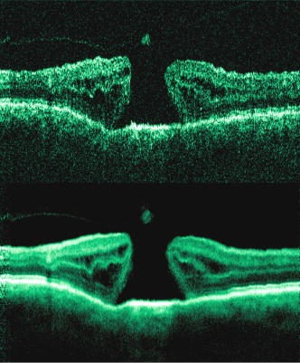

To quantify the improvement in SNRs, we have applied¹⁹ an adequate contrast-to-noise ratio $\left(\mathit{CNR}\right)$ to two neighboring image areas ${\Omega }_1$ and ${\Omega }_2$ with different mean intensities ${\overline{I}}_{{\Omega }_1}$ and ${\overline{I}}_{{\Omega }_2}$ , respectively, and with corresponding standard deviations ${\sigma }_{{\Omega }_1}$ and ${\sigma }_{{\Omega }_2}$ :

Fig. 8

OCT scans from a healthy subject. (top) A single scan in which the image centration at the fovea is perfect as seen from the high-reflecting spot in the fovea (white arrow). (bottom) Average of 14 images after vertical and horizontal registration. Highly reflecting layers in the inner retina are the nerve fiber layer (RNFL), the inner plexiform layer (IPL), and the outer plexiform layer (OPL). Highly reflecting layers in the outer retina are the junction of inner and outer photoceptor segments (IS/OS) and the retinal pigment epithelium (RPE). Approximately $10\mu \mathrm{m}$ anterior to the IS/OS white line is a shallow line representing the external lining membrane (EXL). The nuclear layers are relatively low reflecting, the uppermost nuclear layer is the ganglion cell layer (GCL) followed by the inner nuclear layer (INL) and the outer nuclear layer (ONL). The layer of outer photoreceptor segments (OS) is clearly visible in the fovea.

8.

Clinical Applications

The registration procedure has been tested and used on both healthy subjects and patients with a wide range of pathologies and has shown very encouraging results. Fig. 8 (below) shows the enhancement obtained for a healthy subject and the succeding examples focus on different pathologies including quantitative analysis of macular hole patients. The abbreviations used throughout the case decriptions are: RNFL—retinal nerve fiber layer; GCL—ganglion cell layer; IPL—inner plexiform layer; INL—inner nuclear layer; OPL—outer plexiform layer; PL—photoreceptor layer (nuclei); EXL—external limiting membrane; IS/OS—inner segment/outer segment junction; OS—outer segments; and RPE—retinal pigment epithelium layer.

8.2.

Diabetic Macular Edema

Approximately 20% of diabetic patients develop macular edema with time, ranging from subtle increased thickness to large, diffuse edema including all retinal layers.²⁰ Incipient edema is hard to detect clinically, and OCT has found widespread use for this purpose both for screening and for diagnosis. The leakage originates from the retinal capillaries in the inner retina and diffuses toward the outer PL layer.^{21, 22} Retinal capillaries are hard to visualize with OCT due to low reflectance, although they do give a shadow beneath. Figure 9 shows a fundus image and a combined OCT image for a patient with moderate edema in the foveal center. In these images, the vessel trunks from the superficial retinal vessels are seen dipping down in the superficial capillary plexus and the deeper plexus at the level of the IPL/INL. When the horizontal alignment is included in the average image, the vessels are clearly visible, and as mentioned, the fluid accumulation is found away from the capillaries, in the photoreceptor layer. The mechanism behind this redistribution is not known in detail, and until now, no method has been available for evaluation of the relation between the morphological appearance of the edema and the effect of treatment.^{23, 24}

Fig. 9

(a) Fundus image from a $35\text{-}\text{year}$ -old diabetic patient with a near normal visual acuity $(20∕25)$ . The vertical line shows the position of the OCT scans. Note that the scan line crosses many vessels as well as the small bleeding in the foveal center (partly covered by the arrow). (b) Averaged OCT images. The right side corresponds to the arrowhead in Fig. 9a. (top) Images aligned only by vertical registration. The usual thinning of the fovea is absent, i.e., a clinically significant macular edema is present although it was not detectable by the ophthalmological examination. Just left to the foveal center, a small bleeding gives a spot of hyperreflectance (white arrow). Also, a few of the retinal vessels are seen as hyperreflective trunks leading from the superficial vessels to the capillary plexus deeper in the retina, and below each of these a shadow is seen (white arrow to the left). (bottom) The average image obtained when the image registration includes horizontal shifting. From histology, we know that there are two primary levels for the capillary networks as indicated here, where the trunks go to different layers (white arrow to the left for the lower layer and repeated white arrow for the upper layer). The number of visible vessels have increased compared to the top image, and the borders of the vessels and the shadows are sharper, illustrating the benefit of including the horizontal registration.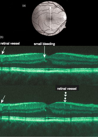

In later stages, with diffuse edema, the edema is also found in the inner retinal layers (see Fig. 10 ). Cystic spaces are seen in the fovea, in the layer of photoreceptor nuclei and the overlying Henles fibers. Cystic spaces are also seen in the surrounding perifoveal region confined to the INL layer, and although the perifoveal cysts are smaller than the central foveal cysts, their presence is probably an indication of a less-favorable visual prognosis compared to patients without cystic spaces in the perifovea. Compared to the average image, the layer of cystic spaces in the INL layer in the single B-scan is less recognizable. On the other hand, the vertical boundaries of the cysts are slightly blurred in the average image due to the decrease in transverse resolution. But most noticeable, the presence of the EXL membrane and the junction of IS/OS segments are not visible in the single B-scan. If the outer retinal layers are absent, the visual prognosis is also unfavorable. In severe cases as this one, a serious detachment is seen in the fovea, just above the RPE.

Fig. 10

Single (top) and average (bottom) OCT images for a $55\text{-}\text{year}$ -old diabetic patient with a marked decrease in visual acuity and a diffuse cystic edema. The cystic spaces are prominent in the center, i.e., in the PL layer/Henles layer, and in addition smaller cysts are seen in the perifoveal INL (white arrows). Just in the center, a serous detachment is seen above the RPE, indicating that the patient has a late-stage macular edema (stippled white arrow). In the average image, both the EXL and the IS/OS junction of the photoreceptors are clearly visible (gray arrows).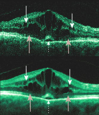

Macular holes can be closed surgically with a large improvement in visual acuity, the prognosis being related to the size of the hole and probably also to other morphological details such as the degree of cystic formation at the edge of the hole. OCT is of major interest here. The enhancement of the OCT images obtained by the registration procedure has found an important clinical applicability in the evaluation of retinal conditions after surgery for idiopathic macular hole where central vision often remains compromised²⁵ (see Fig. 11 ). Since restoration of visual function after macular hole closure clearly depends on a remaining PL layer rather than the clinical observable macular surface configuration, visualization of outer retinal layers is important. Especially, visualization of the IS/OS integrity is an important indicator for photoreceptor survival. Since the denoised average OCT images enhance the visibility of the signals from the PL and RPE layers, quantitative analysis of central photoreceptor defects²⁶ that may be present after macular hole surgery is facilitated. A clinical study is ongoing to evaluate the correlation between visual acuity and photoreceptor defects being quantified from enhanced OCT images.

Fig. 11

(top) Single B-scan $12\text{months}$ after surgery for an idiopathic macular hole. The image primarily allows qualitative analysis of retinal morphology: the macular hole is closed and the reflection from the outer retinal layers is irregular. (bottom) Enhanced OCT scan (based on 8 single scans). The outer retinal layers are clearly discernible, although the normally smooth reflection line from the IS/OS layer is corrupted. The width of the central defect is $475\mu \mathrm{m}$ (dotted white line) corresponding to the marked decrease of visual acuity $(20∕80)$ , which is better than before surgery $(20∕200)$ although not completely satisfactory.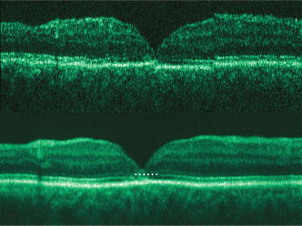

Table 1

Contrast-to-noise ratio (CNR) as a function of the number of images used to produce the average image. Here, shown for two series of registrations.

No. ofRegisteredImages	CNR (ImageSequence 1)	CNR (ImageSequence 2)
1	4.7	4.2
2	5.8	6.9
3	7.1	10.6
4	8.9	11.7
5	8.0	13.4
6	10.0	16.0
7	10.0	16.8
8	10.7	16.8
9	11.4	17.5
10	11.4	16.4
11	12.1	16.5
12		17.3
13		17.9
14		17.8

9.

Discussion

This paper has demonstrated a novel image registration procedure applicable for retinal OCT B-scans obtained by standard OCT systems used for ophthalmology. The method combines a regularized shortest-path algorithm with an iterative scheme for aligning multiple signals. From the registered images, an average image can be calculated. The resulting suppression of noise (including speckle) produces images of a quality that otherwise can be obtained only using ultra-high-resolution OCT laboratory equipment. The enhanced contrast in the combined images facilitates image diagnostics and quantization of pathologies.

In the vast majority of clinical patients, it is possible and feasible to record 12 to 20 images and then manually discard grossly deviating scans. The scans are typically obtained within $5\min$ . Typically around ten scans are left for the alignment procedure. In patients with a substantial loss of vision, this may not be accomplished. Some of these patients also have high levels of retinal scatter, impairing the subjective sorting part where images have to be selected or deselected, and then the combination technique is less powerful.

An assumption of the implemented alignment procedure is that the macroscopic anatomy of the retina does not change significantly with transverse shifts over 30 to 40 microns (due to movement of consecutive tomograms). Naturally a certain loss of resolution cannot be avoided, as also can be observed from the average images. On the other hand, the improvement in SNR is in general so high that more retinal details actually are visible in the average image compared with the single recordings.

The present implementation of the registration algorithm has been implemented in $\mathrm{C}++$ and the registration (both horizontal and vertical) of 10 images takes around $5\min$ on a $3.2\mathrm{GHz}$ Pentium 4. Optimization of the code with respect to the processing time has not been performed.

For macular edema, photocoagulation treatment is the proven treatment, although it is well known that the treatment is not always effective, and new treatments are now in ongoing clinical studies. A possible reason for the slow development in this field is our limited understanding of the stages of severity, leading to poor results in clinical studies and in the evaluation of the individual patient. The methods presented here give improved possibilities for classification based on the retinal morphology by itself.

The enhanced OCT images are also useful when visual acuity is below that expected with no obvious cause. Edema is easy visualized with standard software, but intraretinal defects like atrophy of the outer photoreceptor layers and/or increased backscatter from the outer photoreceptor nuclear layers is clearly more visible with higher SNR, as in the enhanced images presented here.

Although ultra-high-resolution OCT systems give a better resolution,²⁷ these systems will not be available for most ophthalmological departments in the near future. In clinical setups, OCT systems are now used extensively, and for difficult cases and research, the presented contrast enhancement obtained with images from commercial instruments is highy useful. Recently, an eye-tracking system has been combined with the [Humphrey-Zeiss] OCT II commercial system (second-generation time-domain) in order to significantly reduce the registration error relative to the planned transverse scanning path.²⁸ With such a system, one needs only to perform the axial registration when combining a series of recordings to form the average image. Although the average/registration procedure is likely to have most impact on “slow” speed (time-domain OCT) and low-resolution OCT systems, the technique described here can still be beneficial for enhancing the contrast in images obtained using the new generation of Fourier domain OCT systems.