
|
|
1.IntroductionOptical coherence tomography (OCT) is a rapidly emerging medical imaging technology that has applications in many clinical specialties. OCT uses retroreflected light to provide micron-resolution, cross-sectional scans of biological tissues.1, 2, 3 In ophthalmology, OCT is a powerful medical imaging technology because it enables visualization of the cross-sectional structure of the retina and anterior eye with higher resolutions than any other noninvasive imaging modality. Furthermore, OCT image information can be quantitatively analyzed, enabling objective assessment of features such as alterations of the vitreo-retinal interface,4 macular edema,5, 6 retinal nerve fiber layer thickness,7, 8, 9 choroid-nerve head boundary,10 and the extent of the optic cup.11 One of the great advantages of OCT technology is the ability to differentiate various cellular layers of the retina by their optical density.12 In the clinical routine, measurement of retinal thickness by the OCT software depends on the identification of the internal limiting membrane and the hyper-reflective band believed to correspond to the retinal pigment epithelium (RPE)-choriocapillaris interface (or, more precisely, the photoreceptor inner-outer segment border in the case of third generation OCTs). The OCT software calculates the distance between these two boundaries across all of the sampled points (usually along six evenly spaced radial lines) and interpolates the retinal thickness in the unsampled areas between these lines. However, once the various layers can be identified and correlated with the histological structure of the retina, it may seem relevant to measure not only the entire thickness of the retina but also the thickness of the various cellular layers. Moreover, measuring the reflectance of the various retinal layers on OCT images may also be of interest. Drexler have shown in in vitro 12 and in vivo 13 studies that physiological processes of the retina lead to optical density changes that can be observed by a special M-mode OCT imaging known as optophysiology. Thus, it also seems rational that quantitative analysis of reflectance changes may provide clinically relevant information in retinal pathophysiology. Several investigators have demonstrated a relatively high reproducibility of OCT measurements. 14, 15, 16, 17, 18, 19 However, quantitative retinal thickness data generated by OCT could be prone to error as a result of image artifacts, operator errors, decentration errors resulting from poor fixation, and failure of accurate retinal boundary detection by the StratusOCT software algorithms. Therefore, the correct image acquisition along with the accurate and reproducible quantification of retinal features by OCT is crucial for evaluating disease progression and response to therapy. Usually, image analysis quality depends largely upon the quality of the acquired signal itself. Thus, controlling and assessing the OCT image quality is of high importance to obtain the best quantitative and qualitative assessment of retinal morphology. At present, the StratusOCT software provides a quality score, identified as the signal strength (SS), but the clinical advantage of this parameter is not really known. The quality score is based on the total amount of the retinal signal received by the OCT system. We note that the SS score should not be used as an image quality score, since it is basically a signal strength score. Stein found that SS outperformed signal-to-noise ratio (SNR) in terms of poor image discrimination.20 SNR is a standard parameter used to objectively evaluate the quality of acquired images. Stein suggested that SS possibly provides insight into how operators subjectively assess OCT images and stated that SS is a combination of image quality (SNR) and uniformity of signal strength within a scan.20 However, additional detail about SS interpretation is not available from the manufacturer because of its proprietary nature. From our experience, if the best attainable image has an SS of less than 6, the potential for images to be missing valuable tissue information increases. On the other hand, certain types of retinal pathology have a propensity to generate poorer-quality images, and it is difficult to determine whether these pathological images are of poor quality, or if these are the best possible quality images that can be acquired in an eye with advanced retinal damage. During the course of scanning patients in our clinic, we have observed several different types of scan artifacts. Some of these artifacts have been observed previously,21, 22 and have been also analyzed in a systematic manner.23 In general, six types of scan artifacts have been identified and classified in two categories:
Recently, it has been demonstrated that the measurement of retinal thickness along with the internal reflectivity of the various cellular layers of the retina can be extracted from the retinal images obtained with the commercial StratusOCT system after applying a novel segmentation algorithm.24 Cabrera 24 have shown that seven retinal layers can be automatically segmented for facilitating the extraction of local reflectance properties and structural information of the retina. Actually, relative internal reflectivity along with thickness information of the various cellular layers of the retina may provide more detailed information about the pathological changes in retinal morphology. The quantification of such pathological changes mediated by abnormal reflectivity patterns could permit both better detection and follow-up of layer injury as well as better understanding of the diseased retina.24, 25 The main purpose of this study is to investigate how local reflectance and retinal thickness measurements extracted with a novel segmentation algorithm24 are affected by potential artifacts related to OCT operator errors and to suggest strategies for the recognition and avoidance of these pitfalls. 2.Methods2.1.SubjectsEight normal subjects (three men and five women, age years) with normal ocular examination and no history of any current ocular or systematic disease were recruited for this study. Informed consent was obtained from each subject after ethics approval was obtained from the Regional Ethics Committee of Semmelweis University. A pathological case with diabetic macular edema (67-year-old patient, OD) was also used to qualitatively illustrate the effect of operator pitfall errors on pathological retinal alterations. All subjects were treated in accordance with the tenets of the Declaration of Helsinki. 2.2.StratusOCT SystemFor imaging purposes, the commercially available StratusOCT unit (software version 4.0; Carl Zeiss Meditec, Inc., Dublin, California) was used. OCT employs the principle of low-coherence interferometry and is analogous to ultrasound B-mode imaging, but it utilizes light instead of sound to acquire high-resolution images of ocular structures.1 More details of its principles of operation and imaging techniques have been previously described elsewhere. 1, 2, 3, 4, 26, 27 In OCT images, the OCT signal strength is represented in false color using the normal visible spectrum scale. High backscatter is represented by red-orange color, and low backscatter appears blue-black. Thus, tissues that have different reflectivity are displayed in different colors on the false color image. It is important to note that OCT image contrast arises from intrinsic differences in tissue optical properties. Thus, the coloring of different structures represents different optical properties in the false-color image and is not necessarily different tissue pathology. 2.3.Scanning Procedures and Operator Pitfall GenerationA single operator collected all scans per subject in one session. An internal fixation light was used. Since thickness topographic maps depend on accurate determination of retinal thickness in each underlying B-scan, errors in boundary detection in one or more of the six line scans obtained with the radial lines protocol will lead to errors in the calculated macular thickness and volume. Thus, instead of acquiring 6 radial B-scans per subject in each experimental condition, only a single B-scan per modeled artifact and optimal scan acquisition was acquired to simplify the quantitative data analysis. Consequently, a total of 8 and 32 horizontal B-scans (7-mm long, horizontal line scan protocol) were obtained under optimal scan acquisition and specific error’s operator-related artifacts, respectively. Thus, a total of 40 OCT images (B-scans) were obtained and used in the quantitative analysis. The error’s operator-related artifacts included: defocusing, depolarization, decentration, and a combination of defocusing and depolarization. First, an optimal scan was acquired with fine adjustment of the focus and automatic optimization of polarization by the StratusOCT software. Quality assessment of each initial scan (i.e., of each optimal scan without specific error’s operator-related artifacts) was evaluated by two experienced examiners (GMS and DCF). A good-quality scan had to have an even distribution of the signal across the full width of the B-scan, adequate signal strength20 , correct alignments, and no sign of failure of the algorithm for the detection of the inner and outer boundaries of the retina. The manufacturer-provided image assessment parameter (SS) was collected from the OCT data. We note that the SS could be lower than 6 for scans obtained under specific error’s operator-related artifacts, as we could not get a better signal because of the artifact itself. Decentration was modeled by manual movement of the fixation point upward on the StratusOCT interface, resulting in a downward gaze. Thus, the macula would get approximately two optic disk diameters from its original position, as seen on the CCD camera image of the device. The scan line was then manually adjusted to run through the center of the macula. After, macular fixation was repeated and the scan line readjusted to intersect the foveal center. Defocusing was achieved by turning the focus knob diopters. As a next step, image focusing was readjusted and depolarization was achieved by enhancing polarization by clicking 10 times on the increasing button on the StratusOCT interface. For the effect of both artifacts, the focus was then simultaneously turned diopters to achieve defocusing and depolarization. 2.4.Image AnalysisThe OCT raw data was exported to a compatible PC and analyzed using an automated computer algorithm of our own design capable of segmenting the various cellular layers of the retina. Since OCT images suffer from a special kind of noise called “speckle,”28 which poses a major limitation on OCT imaging quality, the OCT raw data was preprocessed. Specifically, we used a model-based enhancement-segmentation approach by combining complex diffusion and coherence-enhanced diffusion filtering in three consecutive steps.24 In particular, the enhancement-segmentation approach starts with a complex diffusion process, which is shown to be advantageous for speckle denoising and edge preservation.24, 29 A coherence-enhanced diffusion filter is then applied to improve the discontinuities in the retinal structure (e.g., gaps created by intraretinal blood vessels) and to obtain the structural coherence information in the raw data.24, 30 The enhancement segmentation approach ends with the application of a boundary detection algorithm based on local coherence information of the structure.24 The new algorithm searches for peaks on each sampling line instead of applying conventional thresholding techniques. The structure coherence matrix is used in this peak finding process instead of the original data. In our peak finding procedure, the peak is identified at the point where the first derivative changes sign from either positive to negative or negative to positive. A total of 7 layers [retinal nerve fiber layer (RNFL); ganglion cell layer (GCL), along with the inner plexiform layer (IPL), inner nuclear layer (INL), outer plexiform layer (OPL), and outer nuclear layer (ONL); photoreceptor inner/outer segment junction (IS/OS); and the section including the retinal pigment epithelium (RPE), along with the choriocapillaries (ChCap) and choroid layer] were automatically extracted using this new approach.24 Once the various cellular layers of the retina were automatically segmented, the relative reflectance and thickness of these layers at the individual points (i.e., at each of the 512 A-scans) were averaged to yield a mean “raw” measurement of thickness and reflectance per layer. We note that the absolute reflectivity can vary according to a wide variety of factors, such as media opacity or scan technique. Thus, each value was a percentage of the local maximum, allowing comparison of different scans in the same patient or subject or even among different patients, different operators, or different OCT machines. Thickness and relative reflectance data were recorded along with mean relative reflectivity deviation from normal (the latter two expressed in %). 2.5.Image Segmentation AccuracySince we are using a new technique of performing image segmentation, a metric geared toward only segmentation needs to be utilized. Thus, an accuracy measure was introduced to evaluate the performance of the new segmentation algorithm. Let us assume that an image obtained from a healthy subject under the optimal scan test is presented to the new segmentation algorithm. The segmentation algorithm then produces a segmented image with detected boundaries depending on which layers were segmented. At this point, we have the correctly segmented image (the “true” segmentation), assuming that no segmentation errors were observed for any layer segmented under the optimal scan procedure. Let us assume now that a second image obtained for the same healthy subject under a specific error’s operator-related artifact is presented to the new segmentation algorithm. The segmentation algorithm then produces a segmented image with detected boundaries , depending on which layers were segmented. Then, assuming that we obtain a segmented image with potential errors in the segmentation, we can measure the performance of the segmentation algorithm per layer by using the following segmentation accuracy measure : where is the total number of boundary pixels detected in the correctly segmented image (i.e., the “true” segmentation). is the number of boundary pixels detected in the segmented image with potential segmentation errors that account for the maximum coverage of the boundary pixels in the “true” segmented image. Note that the maximum coverage measure is actually the fraction of the boundary pixels in the “true” segmented image occupied by the boundary pixels detected in the segmented image with potential segmentation errors. We can measure the overall segmentation accuracy given by the minimum accuracy (i.e., the worst performance) with which individual layers have been identified, i.e., by:The effect of this accuracy measure is illustrated here using an example. Let us assume that two OCT images are obtained from a healthy subject and presented to the segmentation algorithm. One of them is obtained under the optimal scan procedure (i.e., the “true” segmentation image), and the other is acquired under a specific error’s operator-related artifact (i.e., the image with potential segmentation errors). We note that the total number of pixels along each segmented boundary is 512 because there are 512 A-scans in a B-scan (i.e., along the transverse direction). Thus, for each boundary identified on the “true” segmented image. Let us also assume that three retinal boundaries ( , , and ) are segmented on each image. For the retinal boundaries identified on the “true” segmented image ( , , and ), consisting of 512 boundary pixels (i.e., ), the maximum coverage for is provided in the image with potential segmentation errors by a total of 425 boundary pixels (i.e., ), giving [see Eq. 1]. The next boundary to be considered is , for which a maximum coverage of 403 boundary pixels is provided in the image with potential segmentation errors, giving . The third boundary is identified by 320 boundary pixels, giving . The overall accuracy measure, given by the minimum of the three boundaries’ measures, is therefore 0.62 [see Eq. 2]. The accuracy measures were obtained for all the images acquired under a specific error’s operator-related artifacts (i.e., for 32 B-scans). All of the images were then segmented and subsequently verified by eye to identify the algorithm’s failures. Then, the maximum coverage of boundary pixels on each boundary detected on the “true” segmented image was calculated by point-wise comparison with the boundary pixels detected on each boundary extracted on the images obtained under operator pitfall generation. The most accurate segmented image would be one that segments the image with the highest SAM and assigns every pixel in the boundaries identified to the corresponding pixels identified in the “true” segmented image. We note that to obtain the average overall segmentation accuracy values [average , see Eq. 2] for each error’s operator-related artifacts, the accuracy measures per boundary were first calculated for every subject under each specific error’s operator-related artifacts. Then, the minimum accuracy [ , see Eq. 2] with which individual boundaries were identified was obtained for every subject under each specific error’s operator-related artifacts. After that, the average minimum accuracy (average ) was obtained for each specific error’s operator-related artifacts. As a result, a total of 7 segmentation accuracy measures and one minimum accuracy measure were obtained per subject. Thus, a total of 8 values for each error’s operator-related artifacts was used to calculate the final average values. 2.6.Statistical AnalysisFor the statistical analyses of signal strength (SS), thickness, and relative reflectivity data, the Friedman analysis of variance was used.31 In the case of a significant result, Dunnett post hoc analysis was performed in order to reveal the difference from the optimal scan test results. If there was more than one significant difference from the optimal scan test, Newman-Keuls post hoc analysis was also performed.31 Statistica 7.0 software was used (StatSoft, Inc., Tulsa, Oklahoma) in all the statistical analyses performed, and was considered statistically significant. 3.ResultsThe SS score obtained under the optimal image acquisition procedure and each error’s operator-related artifacts procedure is shown in Fig. 1 . Friedman ANOVA and Dunnett post hoc analysis showed significant difference compared to the optimal acquisition protocol in all groups ( in all cases). In order to reveal intergroup changes, additionally, Newman-Keuls post hoc analysis was performed. All groups showed a significant difference compared to each other (data not shown) except for the comparison of decentration with defocus and depolarization ( and , respectively). Fig. 1Distribution of the manufacturer-provided image assessment parameter (SS) for each specific error’s operator-related artifact procedure. Data are represented as mean SD.  Figures 2 and 3 show the StratusOCT images obtained for the optimal image acquisition procedure and each error’s operator-related artifacts procedure in a normal and pathologic subject, respectively. These images with modeled artifacts related to operator errors are particularly shown here to qualitatively illustrate the effect of image acquisition pitfalls on image quality. The pathologic subject was a patient with diabetic macular edema showing multiple lesions located under the fovea. Note the changes in internal reflectivity between the optimal acquisition and operator pitfall procedures. Specifically, note the uneven distribution of signal strength across the full width of the scans obtained under the error’s operator-related artifacts. Interestingly, the retinal lesion located under the fovea appears reduced in size for the decentration process [see Fig. 3e]. As a matter of fact, the cyst appears smaller by decentrating the scan, since the scan line does not cross the same point exactly any more, as with macular fixation. The operator actually took the scan at a different point on the macula [i.e., the scan was a few microns off from the spot targeted in the normal case shown in Fig. 3a]. In general, the retinal images generated with the operator pitfalls showed some reduction in the foveal pit’s curvature, along with a slightly wavy or undulating appearance and loss of retinal structure information across the whole scan length. For example, note that the case illustrated in Fig. 2d shows some loss of retinal structure information as a result of the errors in image acquisition. Fig. 2StratusOCT images obtained for the normal image acquisition procedure and each error’s operator-related artifact procedure for a normal eye (OD). (a) Image obtained with the optimal image acquisition procedure; (b) image obtained with the defocusing procedure; (c) image obtained with the depolarization procedure; (d) image obtained with the combination of defocusing and depolarization procedures; and (e) image obtained with the decentration method. The inner and outer retinal boundaries determined by the StratusOCT built-in algorithm are marked in white. The OCT signal strength is represented in false color using the normal visible spectrum scale. High backscatter is represented by red-orange color and low backscatter appears blue-black. Note the uneven distribution of signal strength across the full width of the images obtained under each error’s operator-related artifacts. 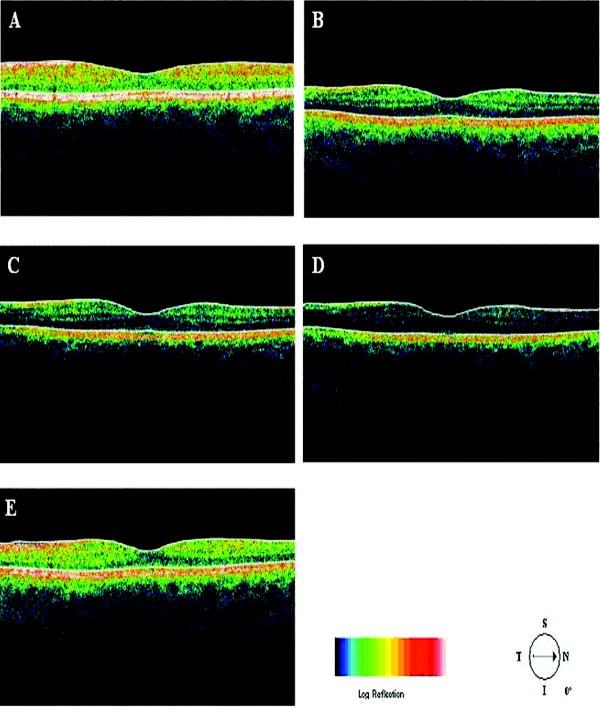 Fig. 3StratusOCT images obtained for the optimal image acquisition procedure and each error’s operator-related artifact procedure for a pathologic eye with diabetic macular edema (OD). (a) Image obtained with the optimal image acquisition procedure; (b) image obtained with the defocusing procedure, (c) image obtained with the depolarization procedure; (d) image obtained with the combination of defocusing and depolarization procedures; and (e) image obtained with the decentration method. The inner and outer retinal boundaries determined by the StratusOCT built-in algorithm are marked in white. Note that the retinal lesions located under the fovea appear reduced in size for the decentration process [see Fig. 3e]. Also note that the built-in algorithm failed to detect the inner layer of the retina [first layer outlined in white from the vitreous (ILM)] for the depolarization case [see the white arrow in Fig. 3c].  Figure 4 shows the results obtained for one of the subjects after applying the automated computer algorithm of our own design capable of segmenting the various cellular layers of the retina.24 Figure 5 shows the segmentation results obtained under the optimal scan acquisition and each error’s operator-related artifacts procedure. The results revealed are for the same subject shown in Fig. 4. The same methodology was used for all the remaining subjects in order to obtain the relative reflectance properties and thickness measurements of the intraretinal layers. Fig. 4Speckle denoising and automated segmentation results. (a) Original OCT image. (b) Denoised image obtained after applying the nonlinear complex diffusion filter and the coherence-enhanced diffusion filtering. (c) Original OCT image with overlaid retinal boundaries. The segmented retinal layers are, from top to bottom, the retinal nerve fiber layer (RNFL), the ganglion cell layer (GCL) along with the inner plexiform layer (IPL), the inner nuclear layer (INL), the outer plexiform layer (OPL), the outer nuclear layer (ONL), and the photoreceptor inner/outer segment junction (IS/OS). The retinal pigment epithelium (RPE) along with the choriocapillaries (ChCap) and choroid layer appear below the bottom boundary line (outlined in green). The OCT images displayed are grayscale representations of the actual interference signal intensities. We note that the sublayer labeled as the ONL is actually enclosing the external limiting membrane (ELM) but in the standard 10 to resolution OCT image, this thin intraretinal layer cannot be visualized clearly. Thus, this layer classification is our assumption and does not reflect the actual anatomic structure. (d) Intraretinal layers and boundary specifications. A total of seven boundaries were detected by the new algorithm. Note that RNFL is bounded by the internal limiting membrane (ILM) and the inner boundary of the GCL . The GCL+IPL complex is bounded by the inner boundary of the GCL and the outer boundary of the IPL . The INL is bounded by the and boundaries. The OPL is bounded by the and boundaries. The ONL is bounded by the and boundaries. The IS/OS layer is bounded by the and boundaries.  Fig. 5Segmentation results obtained for the optimal image acquisition procedure and each error’s operator-related artifact procedure for a normal eye (the same eye shown in Fig. 4). (a) Results for image obtained with the normal image acquisition procedure; (b) results on image obtained with the defocusing procedure; (c) results for image obtained with the depolarization procedure; (d) results for image obtained with the combination of defocusing and depolarization procedures; (e) results for image obtained with the decentration method (note the errors in the detection of the layers); and (f) original raw image.  Of the 32 B-scans with specific error’s operator-related artifacts, 27 exhibited segmentation errors (84.37%). The lowest and highest segmentation error rate was observed under defocus artifact (9.37%) and depolarized-defocus artifact (25%), respectively. Segmentation error locations were also different for each modeled artifact. We note that segmentation errors were not present in the 8 B-scans obtained under the optimal scan acquisition procedure. Table 1 shows the average overall segmentation accuracy measures (average ) obtained per intraretinal boundary and for each specific error’s operator-related artifacts. Note that segmented boundaries with fewer artifacts (i.e., with highest average values) were observed for images obtained under defocus and decentration artifacts (see Table 1). Moreover, inner and outer retina misidentification artifacts were not observed under any error’s operator-related artifacts [see values obtained for ILM, ONLo (OCT frequent used outer limit), and (redefined outer limit) boundaries in Table 1]. Thus, these particular boundaries were in very good agreement point-wise with the boundaries detected on images obtained under the optimal scan acquisition procedure. However, the , , and boundaries showed the worst segmentation performance in all the pitfall cases tested (see Table 1). Table 1Segmentation accuracy measures (average SAMoverall values) obtained after comparing the segmentation result on modeled artifacts’ images with the “true” segmentation.
Table 2 shows the mean and standard deviation results per layer along with statistical analysis results for both thickness and relative reflectivity. Figure 6 shows the mean relative reflectivity values obtained per layer. Note the marked reduction in internal reflectivity per layer for all the pitfall cases generated in comparison with the mean values obtained under the optimal acquisition procedure. A significant difference from the optimal reflectivity was observed for complex under the depolarization-defocus artifact, which is in agreement with the lowest average value obtained for (see Table 1). We note that the complex is bounded by the and boundaries [see Fig. 4d]. A marked although statistically not significant decrease in mean relative reflectivity was observed due to depolarization artifact in all layers, while defocus resulted in a less-marked decrease. In general, decentration and defocus both had a similar altering effect on all reflectivity measurements (see Fig. 6 and Table 2). The average thickness for each layer segmented is shown in Fig. 7 and Table 2. In this case, a greater—although statistically not significant—effect of depolarization was observed on measurements compared to defocus. However, a statistically significant difference in average thickness was found for depolarization-defocus in the case of the complex and ONL layer segmentation ( ; see Table 2). This particular result is in agreement with the lowest average values obtained for the and boundaries (see Table 1). We note that the ONL is bounded by the and boundaries [see Fig. 4d]. As can be seen, the two artifacts together (depolarized-defocus) had the greatest statistically significant altering effect on all measurements (see Fig. 7, Table 1, and Table 2). Decentration had a comparable effect on thickness measurements, however, not reaching statistical significance. These results demonstrate how the accuracy of thickness measurements can be degraded by the variability in measured reflectance under artifacts related to OCT operator errors. It is interesting to note that depolarization resulted in a bigger, significant reduction in SS than defocusing alone, while the combination of the two resulted in an even more pronounced reduction in SS (see Fig. 1). Correspondingly, both reflectance and thickness data were more influenced by depolarization, and most influenced by the combination of the two. Fig. 6Mean relative reflectivity values obtained per layer. For SD values and statistical analysis results, see Table 2.  Fig. 7Mean thickness values obtained per layer. Note that a clear thinning and thickening effect was obtained for the complex and the ONL, respectively. For SD values and statistical analysis results, see Table 2.  Figure 8 shows the mean relative reflectivity’s deviation from the optimal image’s mean values. The mean relative reflectivity deviation from the norm showed the highest variation for the complex (10 to 23% deviation), followed by the OPL (8 to 14%), INL (6 to 12%), and RNFL (8 to 13%). It is important to point out that the low spatial resolution of StratusOCT compared to the ultra-high resolution OCT devices is not in itself a pitfall but should be kept in mind because differentiation between intraretinal layers with low backscattering becomes difficult if not impossible under such pitfalls. Fig. 8Mean relative reflectivity deviation from the optimal image’s mean values. Note that the two artifacts together (depolarized-defocus) had the greatest altering effect on all measurements. 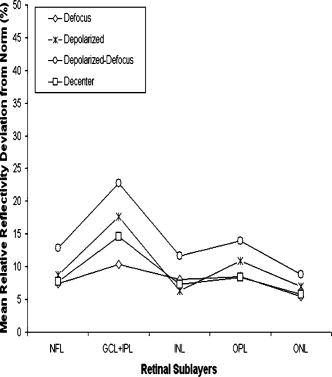 Finally, we would like to mention that the retinal thickness values provided by the StratusOCT mapping software should be carefully reappraised. For example, due to the operator pitfall errors, the StratusOCT custom built-in algorithm failed to locate properly the inner and outer boundaries of the retina [see Fig. 9a ]. Since these boundaries are found by a threshold procedure, their estimated locations could be sensitive to relative differences in reflectance between the outer and deeper retinal structures. Thus, even scans of normal eyes could have inner and outer retina misidentification artifacts under operator errors. The segmentation result using our methodology is also shown for comparison, properly identifying the retinal boundaries [see Fig. 9b and the values in Table 1 for the ILM and the ONLo boundaries]. Also, note that the built-in algorithm failed to detect the inner layer of the retina (first layer outlined in white from the vitreous) for the depolarization case in the pathologic eye [see Fig. 3c]. Fig. 9Segmentation results showing the performance of the StratusOCT custom built-in algorithm compared to the results using our custom algorithm. (a) Macular scan obtained for eye 3 under the depolarization artifact. Note the misidentification of the outer boundary of the retina (outlined in white). (b) Results obtained for the same eye (eye 3, depolarization error) using our methodology. Note that our algorithm was able to correctly detect the outer boundary of the retina.  Table 2Mean and standard deviation results per layer compared to optimal scan acquisition conditions (Friedman ANOVA followed by Dunnett post hoc analysis; NS not significant; † p<0.05 compared to normal).
4.DiscussionIn this study, the presence and severity of segmentation errors by a novel segmentation algorithm was evaluated under potential OCT image acquisition pitfalls. Our results showed that defocusing and depolarization errors together have a substantial effect on the quality and precision of information extracted from OCT images by using the novel algorithm. As stated in the Sec. 3, the , , and boundaries were more prone to segmentation errors under the modeled image acquisition pitfalls. The lowest segmentation accuracy was achieved by the combined depolarization-defocus artifact (see the average values in Table 1), and accordingly, significant changes in relative reflectivity and thickness were due to this type of artifact. An awareness of these pitfalls and possible solutions is crucial not only for avoiding misinterpretation of OCT images but also for assuring the quality of the quantification of retinal measurements. It is important to note that visual analysis of OCT image quality is affected by intraretinal abnormalities in backscattering that are usually associated to particular ocular diseases. Thus, optimal settings are necessary to avoid measurement errors. For example, the StratusOCT built-in algorithm requires clear delineation of the inner and outer retinal boundaries to accurately identify intraretinal abnormalities. It is well known that StratusOCT images are prone to error as a result of inner or outer retina misidentification artifacts. However, our segmentation results for the inner and outer retinal layers showed no misidentification errors for any modeled artifact. Thus, the new segmentation algorithm could provide a more reliable macular volume and thickness measurement than the OCT built-in algorithm under the error’s operator-related artifacts. Further study is needed with a larger sample size to validate these preliminary results and obtain the reproducibility of the retinal measurements extracted by using the novel algorithm. As a result of this work and taking into account our experience during the course of scanning a large number of patients per year in our clinic, a few comments are in order about specific strategies for the recognition and avoidance of image acquisition pitfalls. In order to avoid potential image acquisition pitfalls, it is necessary that first the operator assure the correct placement of the patient’s head on the chin- and headrest of the StratusOCT system. Moreover, it is imperative that the lateral canthus markers be lined up with the center of the pupil in primary gaze. Second, polarization optimization must be done before and may be repeated during a scanning session. For example, in the case of a radial line scan that is composed of six consecutive scans, the operator should polarize before obtaining the first scan and then may have to repeat polarization for the fourth and sixth scan if needed. On the other hand, opacities in the eye or corneal drying may change the signal strength on one scan and not the other, requiring the operator to repolarize. It is also worth mentioning that a target is deemed desirable in identifying a potentially good-quality scan,20 although it is not always possible because of factors such as media opacity. Significant changes in relative reflectance and thickness were observed under the combined defocus-depolarization artifact where SS was below the above-mentioned level, which reinforces our theory. For instance, dense cataracts and vitreous opacities limit the image quality no matter how well centered and adjusted the scan. We also note that an ideal scan will have an even SS level across the entire scan, with no sections of weak signal. Furthermore, it is crucial that the operator centers all six scans at the fovea when acquiring macular scans for retinal thickness analysis. This is a problem for patients that have poor fixation due to impaired visual acuity. We note that average thickness and standard deviation of the retinal thickness at the fovea is automatically calculated by the retinal map (single eye) or retinal thickness/volume (OU) analyze protocols. These protocols use the central A-scan of each one of the six radial scans (B-scans) obtained during the acquisition session to calculate foveal thickness. In theory, all six radial scans (B-scans) are to be centered at the same point (fovea) after a perfect acquisition session. Thus, the central A-scan should be the same for all six B-scans, and the standard deviation of the retinal thickness at the fovea has to be equal to zero. Depending on the distortions of the macular morphology associated to the disease, standard deviation values of the average foveal thickness higher than (or an of central retinal thickness)23 are highly indicative that at least one of the six radial scans is not correctly centered at the fovea. Consequently, a new entire scan acquisition session should be performed. Although it may seem unusual, the correct focus is not necessarily one that the operator appreciates in the fundus image but one that the operator appreciates in the greater intensity of color saturation in the current scanned image. Thus, it is more important to have a good scanned image than it is to have a good fundus image. The laser and the fundus video camera are not on the same plane, so when one has the best view in one image, the other may not have the same quality. As can be seen, an awareness of all these pitfalls is crucial when misinterpretation is to be prevented, which may be important in the planning and evaluation of further studies using the new segmentation algorithm. Moreover, it is important for the use of the new algorithm that physicians be able to trust measurements such as thickness maps of the intraretinal layers and macular thickness and volume. This emphasizes the goal of our present work for future studies. AcknowledgmentsThis study is supported in part by Grant No. NIH R01 EY008684-10S1, by NIH Grant No. P30-EY014801, by an unrestricted grant to the University of Miami from Research to Prevent Blindness, Inc., and by a PhD fellowship grant at Semmelweis University, School of PhD Studies (Grant No. 2/10). The authors appreciate helpful discussions with Mr. Carl E. Denis, ophthalmic photography specialist from the Bascom Palmer Eye Institute. Carmen A. Puliafito receives royalties for intellectual property licensed by Massachusetts Institute of Technology to Carl Zeiss Meditec, Inc. ReferencesD. Huang,
E. A. Swanson,
C. P. Lin,
J. S. Schuman,
W. G. Stinson,
W. Chang,
M. R. Hee,
T. Flotte,
K. Gregory, and
C. A. Puliafito,
“Optical coherence tomography,”
Science, 254 1178
–1181
(1991). https://doi.org/10.1126/science.1957169 0036-8075 Google Scholar
J. A. Izatt,
M. R. Hee,
E. A. Swanson,
C. P. Lin,
D. Huang,
J. S. Schuman,
C. A. Puliafito, and
J. G. Fujimoto,
“Micrometer-scale resolution imaging of the anterior eye in vivo with optical coherence tomography,”
Arch. Ophthalmol. (Chicago), 112 1584
–1589
(1994). 0003-9950 Google Scholar
M. R. Hee,
J. A. Izatt,
E. A. Swanson,
D. Huang,
J. S. Schuman,
C. P. Lin,
C. A. Puliafito, and
J. G. Fujimoto,
“Optical coherence tomography of the human retina,”
Arch. Ophthalmol. (Chicago), 113 325
–332
(1995). 0003-9950 Google Scholar
C. A. Puliafito,
M. R. Hee,
C. P. Lin,
E. Reichel,
J. S. Schuman,
J. S. Duker,
J. A. Izatt,
E. A. Swanson, and
J. G. Fujimoto,
“Imaging of macular diseases with optical coherence tomography,”
Ophthalmology, 102 217
–229
(1995). 0161-6420 Google Scholar
M. R. Hee,
C. A. Puliafito,
J. S. Duker,
E. Reichel,
J. G. Coker,
J. R. Wilkins,
J. S. Schuman,
E. A. Swanson, and
J. G. Fujimoto,
“Topography of diabetic macular edema with optical coherence tomography,”
Ophthalmology, 105 360
–370
(1998). https://doi.org/10.1016/S0161-6420(98)93601-6 0161-6420 Google Scholar
M. R. Hee,
C. A. Puliafito,
C. Wong,
J. S. Duker,
E. Reichel,
B. Rutledge,
J. S. Schuman,
E. A. Swanson, and
J. G. Fujimoto,
“Quantitative assessment of macular edema with optical coherence tomography,”
Arch. Ophthalmol. (Chicago), 113 1019
–1029
(1995). 0003-9950 Google Scholar
J. S. Schuman,
M. R. Hee,
C. A. Puliafito,
C. Wong,
T. Pedut-Kloizman,
C. P. Lin,
E. Hertzmark,
J. A. Izatt,
E. A. Swanson, and
J. G. Fujimoto,
“Quantification of nerve fiber layer thickness in normal and glaucomatous eyes using optical coherence tomography,”
Arch. Ophthalmol. (Chicago), 113 586
–596
(1995). 0003-9950 Google Scholar
J. S. Schuman,
M. R. Hee,
A. V. Arya,
T. Pedut-Kloizman,
C. A. Puliafito,
J. G. Fujimoto, and
E. A. Swanson,
“Optical coherence tomography: a new tool for glaucoma diagnosis,”
Curr. Opin. Ophthalmol., 6 89
–95
(1995). Google Scholar
L. Pieroth,
J. S. Schuman,
E. Hertzmark,
M. R. Hee,
J. R. Wilkins,
J. Coker,
C. Mattox,
R. Pedut-Kloizman,
C. A. Puliafito,
J. G. Fujimoto, and
E. Swanson,
“Evaluation of focal defects of the nerve fiber layer using optical coherence tomography,”
Ophthalmology, 106 570
–579
(1999). https://doi.org/10.1016/S0161-6420(99)90118-5 0161-6420 Google Scholar
M. R. Hee,
C. A. Puliafito,
C. Wong,
E. Reichel,
J. S. Duker,
J. S. Schuman,
E. A. Swanson, and
J. G. Fujimoto,
“Optical coherence tomography of central serous chorioretinopathy,”
Am. J. Ophthalmol., 120 65
–74
(1995). 0002-9394 Google Scholar
B. K. Rutledge,
C. A. Puliafito,
J. S. Duker,
M. R. Hee, and
M. S. Cox,
“Optical coherence tomography of macular lesions associated with optic nerve head pits,”
Ophthalmology, 103 1047
–1053
(1996). 0161-6420 Google Scholar
K. Bizheva,
R. Pflug,
B. Hermann,
B. Povazay,
H. Sattmann,
P. Qiu,
E. Anger,
H. Reitsamer,
S. Popov,
J. R. Taylor,
A. Unterhuber,
P. Ahnelt, and
W. Drexler,
“Optophysiology: depth-resolved probing of retinal physiology with functional ultrahigh-resolution optical coherence tomography,”
Proc. Natl. Acad. Sci. U.S.A., 28
(103), 5066
–5071
(2006). https://doi.org/10.1073/pnas.0506997103 0027-8424 Google Scholar
B. Hermann,
B. Považay,
A. Unterhuber,
M. Lessel,
H. Sattmann,
U. Schmidt-Erfurth, and
W. Drexler,
“Optophysiology of the human retina with functional ultrahigh resolution optical coherence tomography,”
(2006) Google Scholar
E. Z. Blumenthal,
J. M. Williams,
R. N. Weinreb,
C. A. Girkin,
C. C. Berry, and
L. M. Zangwill,
“Reproducibility of nerve fiber layer thickness measurements by use of optical coherence tomography,”
Ophthalmology, 107 2278
–2282
(2002). https://doi.org/10.1016/S0161-6420(00)00341-9 0161-6420 Google Scholar
D. J. Browning,
“Interobserver variability in optical coherence tomography for macular edema,”
Am. J. Ophthalmol., 137 1116
–1117
(2004). https://doi.org/10.1016/j.ajo.2003.12.013 0002-9394 Google Scholar
P. Carpineto,
M. Ciancaglini,
E. Zuppardi,
G. Falconio,
E. Doronzo, and
L. Mastropasqua,
“Reliability of nerve fiber layer thickness measurements using optical coherence tomography in normal and glaucomatous eyes,”
Ophthalmology, 110 190
–195
(2003). https://doi.org/10.1016/S0161-6420(02)01296-4 0161-6420 Google Scholar
P. Massin,
E. Vicaut,
B. Haouchine,
A. Erginay,
M. Paques, and
A. Gaudric,
“Reproducibility of retinal mapping using optical coherence tomography,”
Arch. Ophthalmol. (Chicago), 119 1135
–1142
(2001). 0003-9950 Google Scholar
L. A. Paunescu,
J. S. Schuman,
L. L. Price,
P. C. Stark,
S. Beaton,
H. Ishikawa,
G. Wollstein, and
J. G. Fujimoto,
“Reproducibility of nerve fiber thickness, macular thickness, and optic nerve head measurements using StratusOCT,”
Invest. Ophthalmol. Visual Sci., 45 1716
–1724
(2004). https://doi.org/10.1167/iovs.03-0514 0146-0404 Google Scholar
J. S. Schuman,
T. Pedut-Kloizman, and
E. Hertzmark,
“Reproducibility of nerve fiber layer thickness measurements using optical coherence tomography,”
Ophthalmology, 103 1889
–1898
(1996). 0161-6420 Google Scholar
D. M. Stein,
H. Ishikawa,
R. Hariprasad,
G. Wollstein,
R. J. Noecker,
J. G. Fujimoto, and
J. S. Schuman,
“A new quality assessment parameter for optical coherence tomography,”
Br. J. Ophthamol., 90 186
–190
(2006). https://doi.org/10.1136/bjo.2004.059824 0007-1161 Google Scholar
G. C. Hoffmeyer,
“MacPac: a systematic protocol for OCT scanning of macular pathology,”
J. Ophthal. Photograph., 25 64
–70
(2003). Google Scholar
G. J. Jaffe and
J. Caprioli,
“Optical coherence tomography to detect and manage retinal disease and glaucoma,”
Am. J. Ophthalmol., 137 156
–169
(2004). https://doi.org/10.1016/S0002-9394(03)00792-X 0002-9394 Google Scholar
R. Ray,
S. S. Stinnett, and
G. J. Jaffe,
“Evaluation of image artifact produced by OCT of retinal pathology,”
Am. J. Ophthalmol., 139 18
–29
(2005). 0002-9394 Google Scholar
D. Cabrera Fernández,
H. M. Salinas, and
C. A. Puliafito,
“Automated detection of retinal layer structures on optical coherence images,”
Opt. Express, 13 10200
–10216
(2005). https://doi.org/10.1364/OPEX.13.010200 1094-4087 Google Scholar
M. E. Pons,
H. Ishikawa,
R. Gurses-Ozden,
J. M. Liebmann,
H. L. Dou, and
R. Ritch,
“Assessment of retinal nerve fiber layer internal reflectivity in eyes with and without glaucoma using OCT,”
Arch. Ophthalmol. (Chicago), 118 1044
–1047
(2000). 0003-9950 Google Scholar
C. A. Toth,
R. Birngruber, and
S. A. Boppart,
“Argon laser retinal lesions evaluated in vivo by optical coherence tomography,”
Am. J. Ophthalmol., 123 188
–198
(1997). 0002-9394 Google Scholar
M. R. Hee,
“Artifacts in optical coherence tomography topographic maps,”
Am. J. Ophthalmol., 139 154
–155
(2005). https://doi.org/10.1016/j.ajo.2004.08.066 0002-9394 Google Scholar
L. M. Schmitt,
S. H. Xiang, and
K. M. Yung,
“Speckle in optical coherence tomography,”
J. Biomed. Opt., 1 95
–105
(1999). https://doi.org/10.1117/1.429925 1083-3668 Google Scholar
G. Gilboa,
N. Sochen, and
Y. Y. Zeevi,
“Image enhancement and denoising by complex diffusion process,”
IEEE Trans. Pattern Anal. Mach. Intell., 25 1020
–1036
(2004). https://doi.org/10.1109/TPAMI.2004.47 0162-8828 Google Scholar
J. Weickert,
“Coherence-enhancing diffusion filtering,”
Int. J. Comput. Vis., 31 111
–127
(1999). https://doi.org/10.1023/A:1008009714131 0920-5691 Google Scholar
S. Siegel and
N. J. Castellan, Nonparametric Statistics for the Behavioral Sciences, 2nd ed.McGraw-Hill, New York (1988). Google Scholar
|
||||||||||||||||||||||||||||||||||||||||||||||||||||||||||||||||||||||||||||||||||||||||||||||||||||||||||||||||||||||||||||||||


