1.

Introduction

Fourier domain optical coherence tomography (FDOCT) has currently become the method of choice for fast high resolution retinal imaging in 3-D. ^{1, 2, 3, 4, 5}. It offers even at depth profile rates of 10- to 30-kHz high sensitivity to reveal retinal morphology close to the level of histology. ^{6, 7, 8, 9} Novel trends in biomedical imaging aim for functional tissue imaging, including spectroscopic contrast,¹⁰ polarization contrast,^{11, 12} and Doppler flow imaging.^{13, 14} Since the human retina is one of the organs with highest perfusion, any pathology will have an immediate impact on the vascularization and blood supply. Several publications outlined the importance of studying blood flow as an early indicator of various retinal diseases such as glaucoma or diabetic retinopathy.^{15, 16, 17}

Doppler OCT can not only measure tissue perfusion but, compared to laser Doppler flowmetry,¹⁸ has the advantage of providing depth localized blood flow. FDOCT has, in addition, high phase stability and its high acquisition speed allows for 3-D in vivo imaging of retinal vascularization. The achieved image quality can already be compared to that of retinal fluorescence angiography.¹⁹

Doppler OCT measures only the axial component of the flow velocity vector. There have been different approaches in time-domain OCT to obtain the transverse velocity information from OCT signal peak broadening.^{20, 21} In FDOCT, such an approach is difficult to realize. Nevertheless, if one has the full 3-D structure at hand, one can deduce the complete velocity vectors from the direction of the blood vessels within the recorded 3-D volume. Hence the problem has been shifted to the segmentation of the vessel structure and the determination of vessel directions.

Recently we introduced the concept of resonant Doppler imaging.²² The method does not only allow measuring high flow velocities that are not available via standard phase sensitive Doppler FDOCT, it also suppresses the static structure and enhances the contrast for flow signals. As a result, one achieves segmentation of blood vessels without elaborate imaging processing techniques, which is the base for the true velocity vector reconstruction presented.

2.

Theoretical Considerations

Information about blood flow can be extracted from the FDOCT signal phase.²³ The Fourier transform of the spectral interference pattern has a complex result and can be written as ${\widehat{S}}_{FDOCT}\left(z\right)=FT\left\{I\right(k\left)\right\}=\mid {\widehat{S}}_{FDOCT}\left(z\right)\mid exp[-i\phi (z\left)\right]$ , where $I\left(k\right)$ is the interference pattern as function of wavenumber $k$ . The phase itself due to the $2\pi$ ambiguity has no direct meaning. Nevertheless, by using a reference such as any prominent signal at a static interface in the sample arm, one has an ultra-sensitive method at hand to measure distances of some nanometers as well as slight changes in refractive index.²⁴ Also, a temporally earlier depth scan at the same position can serve as a reference, which is the basis for phase-sensitive Doppler FDOCT. If $\tau$ is the period between successive spectra, one can directly calculate the depth resolved axial velocity $v\left(z\right)$ of a moving sample interface from the phase difference of two adjacent depth scans, i.e., $v\left(z\right)=\left[\phi \right(z,t+\tau )-\phi (z,t\left)\right]\lambda ∕\left(4\pi \tau \right)$ , where $\lambda$ is the center wavelength of the light source spectrum. The maximum velocity is, in theory, given according to the sampling theorem for a phase difference of $\pi$ , i.e., $V_{\max }=\lambda ∕\left(4\tau \right)$ .

Although spectrometer-based FDOCT offers outstanding phase stability, it still suffers from interference fringe blurring caused by sample motion.²⁵ This effect leads to attenuation and—depending on the system sensitivity and dynamic range—loss of flow signals. In addition, it has been shown¹¹ that the phase sensitivity is directly related to the signal-to noise ratio (SNR) via $\delta \phi =1∕\sqrt{SNR}$ . Hence, the phase sensitivity will be reduced for detection of flow.

Recently we proposed a different approach to measure flow with spectrometer-based FDOCT, so-called resonant Doppler imaging.²² The idea is to move the detection with the flow signal like a photographer taking a photograph of a moving object. The movement of the detection that counterbalances the sample motion is realized via an electro-optic phase modulator (EOM) in the reference arm. Let us assume a single interface in the sample arm moving at constant velocity $v$ along the optical axis. If the signal integration time is $T$ , one obtains for the interference part of the recorded signal using reference phase shifting^{22, 25}:

From Eq. 1 we observe that the total phase change during camera integration reduces the modulation depth of the spectral interference pattern and leads, after performing the Fourier transform and taking into account the chromaticity of the phase change, to an attenuated FDOCT signal:

From Eq. 2 we immediately see that the signal of the moving sample interface can be completely recovered if the reference velocity $v_{\mathrm{ref}}$ matches the sample velocity $v$ , setting the overall phase change $\mathrm{\Delta }\Phi$ to zero. In Fig. 1a we show the attenuation curves without reference velocity $v_{\mathrm{ref}}=0$ ( $A_{\mathrm{static}}$ solid line), with a positive reference velocity $v_{\mathrm{ref}}$ ( $A_{\mathrm{up}}$ dotted line), and with a negative reference velocity $-v_{\mathrm{ref}}$ ( $A_{\mathrm{down}}$ dashed line). The reference velocity displaces the attenuation curve $A\left(v\right)$ and leads to an attenuation of static signals, whereas moving structures will be enhanced [arrows in Fig. 1a]. This is the essence of optical vivisection of tissue vascularization.²²

Fig. 1

(a) Attenuation curves for different reference velocities $v_{\mathrm{ref}}:A_{\mathrm{static}}$ (solid line) $v_{\mathrm{ref}}=0$ , $A_{\mathrm{up}}$ (dash-dotted line) $+v_{\mathrm{ref}}$ , and $A_{\mathrm{down}}$ (dashed line) $-v_{\mathrm{ref}}$ . For reference shifting, static signals will be suppressed, whereas moving structures will gain contrast (arrows). (b) Difference between the different attenuation curves. Within the shaded region, delimited by $v_{\min }$ and $v_{\max }$ , one can associate unique velocity values to the logarithmic SNR difference.

In addition, we can use the relative attenuation between two recordings with different reference offsets for flow quantification. We consider the overlap regions between two attenuation curves in Fig. 1a. The typical SNR of measured structures will set a limit to the quantifiable velocity range as indicated by the shadowed region, assuming a SNR of $20\mathrm{dB}$ . In Fig. 1b we displayed the logarithmically scaled attenuation curve ratios for all three combinations with opposite reference velocity offsets. Assuming three recordings $\widehat{I}(z_0,v_{ref}=0)$ and $\widehat{I}(z_0,\pm v_{ref})$ , we can write $\mathrm{\Delta }A\left(v\right)=A[v\mp v_{ref}]∕A\left(v\right)=\widehat{I}\left[v\right(z_0),\pm v_{ref}]∕\widehat{I}\left[v\right(z_0),v_{ref}=0]$ . Within the shaded regions, we can attribute a unique sample velocity value to an attenuation ratio as $v=\mathrm{\Delta }{A}^{-1}\left(v\right)$ . In practice we first calculate the ratio between two oppositely shifted depth scans [solid line in Fig. 1b]. The sign of the logarithmically scaled ratio is then used to decide which attenuation ratio curve to use as a look-up table for the actual velocity determination: $A_{\mathrm{down}}-A_{\mathrm{static}}$ (dashed line), or $A_{\mathrm{up}}-A_{\mathrm{static}}$ (dotted line).

3.

Experimental

The optical setup displayed in Fig. 2 is based on a modified Mach-Zehnder configuration. Two superluminescence diodes (EXALOS AG, Switzerland) are combined to yield a full width at half maximum (FWHM) spectral bandwidth of $36\mathrm{nm}$ , a central wavelength of $833.5\mathrm{nm}$ , resulting in an axial resolution of $8.5\mathrm{\mu }\mathrm{m}$ in air. The polarizer is oriented to match the fast axis of the EOM crystal. The light passes in the reference arm EOM (Nova Phase) and is afterward circularly polarized by a quarter waveplate. The dispersion compensation accounts for the optics in the sample arm as well as for the water of the eye bulb. The translation stage allows adjusting the reference arm length to the subject position. In the sample arm, the light passes a $\mathrm{LiNbO}3$ crystal to compensate for the dispersion of the EOM. The telescope L1-L2 expands the beam diameter by a factor of 2.5. The subject eye is illuminated via an $x$ - $y$ scanning stage (Cambridge Technology) and a telescope L3-L4 that has an angular magnification of 2. The beam diameter at the eye is $1.8\mathrm{mm}$ , resulting in a theoretic transverse spot size of $14\mathrm{\mu }\mathrm{m}$ on the retina. The optical power at the cornea is $300\mathrm{\mu }\mathrm{W}$ , which is safe for direct beam viewing according to American National Standards Institute (ANSI) laser safety regulations. The spectral interference pattern between sample and reference arm light is recorded by a spectrometer consisting of a diffraction grating (Wasatch, $1200\mathrm{lines}∕\mathrm{mm}$ ) and a charge-coupled device (CCD) line scan camera (Atmel, Aviiva, 2048 pixels, $12\mathrm{bit}$ ). An objective lens of 135-mm focal length images a spectral bandwidth of $68\mathrm{nm}$ onto the 1024 pixels of the camera, which were actually used for the acquisition. The line rate or equivalent A-scan rate of the camera is $17.4\mathrm{kHz}$ (without processing) with an integration time $\tau$ of $43\mathrm{\mu }\mathrm{s}$ . The maximum depth range in air is $2.6\mathrm{mm}$ . The sensitivity close to the zero delay is $98\mathrm{dB}$ with a decay of $-7\mathrm{dB}∕\mathrm{mm}$ .

Fig. 2

(a) Optical setup: SLD1, 2 are superluminescence diodes; Pol is the polarizer; $\mathrm{LiNbO}3$ is a Lithium-Niobate crystal; EOM is the electro-optic modulator; Ll, L2 is the telescope with $\mathrm{f}=-40$ and $100\mathrm{mm}$ , respectively; $\lambda ∕4$ is the quarter waveplate; Disp is dispersion compensation; TS is the translation stage; L3,L4 is the telescope $\mathrm{f}=60$ and $30\mathrm{mm}$ ; X-Y Sc are galvo scanners; DG is diffraction grating; L5 is the objective $\mathrm{f}=135\mathrm{mm}$ ; and CCD is the line scan camera. (b) Synchronization between camera (Cam) line period T, integration time $\tau$ , and the EOM driving voltage.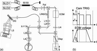

The EOM is driven by an arbitrary function generator (Agilent 33220A), followed by a high voltage amplifier (20x). The phase change introduced by the EOM is $\mathrm{\Delta }{\Phi }_{ref}=\pi \mathrm{\Delta }V∕V_{\pi }$ , where $V_{\pi }$ is the voltage at the EOM that leads to a phase shift of $\pi$ . The associated reference arm velocity at the center wavelength $\lambda$ is $v_{ref}=\mathrm{\Delta }{\Phi }_{ref}\lambda ∕\left(4\pi T\right)$ . The half-wave voltage $V_{\pi }$ is provided by the manufacturer. Figure 2b shows the synchronization of the EOM with the camera integration. It corresponds to a three-stage mode: first, a positive voltage slope of $9.3\mathrm{V}∕\mathrm{\mu }\sec$ is applied to the EOM corresponding to a total phase shift of $\mathrm{\Delta }{\Phi }_{ref}\left(k\right)=2\pi$ , a velocity of $v_{2\pi }=\lambda ∕2\tau =9.7\mathrm{mm}∕\mathrm{s}$ , and an associated Doppler frequency of $23.3\mathrm{kHz}$ . The resolvable axial velocities were $v_{\min }=1\mathrm{mm}∕\mathrm{s}$ and $v_{\max }=9\mathrm{mm}∕\mathrm{s}$ [see Figs. 1a and 1b]. This is followed by a constant voltage level that corresponds to a standard FDOCT tomogram without reference phase shifting, and third a negative voltage slope of the same amount as the positive slope. The three tomogram channels are recorded in an interlaced way during continuous transverse scanning.

4.

Blood Vessel Segmentation and Velocity Vector Determination

The flow velocity extraction methods outlined in Sec. 2 yield only the projection onto the optical axis $v_{\parallel }=v\bullet \cos \alpha$ of the full flow vector $\mathbf{v}=v(\cos \theta \sin \alpha ,\sin \theta \sin \alpha ,\cos \alpha )$ [Fig. 3a ]. Let us assume that the flow direction is parallel to the vessel direction, which is valid for laminar flow. It is then sufficient to determine the actual vessel direction within the 3-D sample volume to obtain the angle $\alpha$ of the flow vector $\mathbf{v}$ with respect to the incident probing beam according to

Fig. 3

(a) Speed $\mathit{v}$ expressed as one component parallel $v_{\mid \mid }=v_z$ and a one perpendicular $v_{\perp }=\sqrt{v_x^2+v_y^2}$ (dashed line) to the optical axis. (b) The observable part of $v_{\mid \mid }$ is restricted by $v_{\min }$ and $v_{\max }$ (shaded region), which involves a restriction of the observable angles $\alpha =\mathrm{atan}(v_{\perp }∕v_{\Vert })$ . We indicate the observable angle range (curved lines) for three different values of $v$ . (c) Angle range (shaded region) as a function of the module of the velocity.

The task is now to identify the vessel structure, to track the orientation within the 3-D volume, and to extract the angle $\alpha$ to the optical axis for finally applying Eq. 3. Figure 4 displays first a standard FDOCT tomogram, together with the Doppler flow map consisting of 2240 transversal points across the foveal region and the optic nerve head along $12\mathrm{mm}$ . For the flow analysis, we concentrated on the indicated region of interest at the optic nerve head (ONH). In this region, flow velocities are fast due to the large vessel diameters on one hand and the strong inclination of the vessels with respect to the optic axis on the other hand. As a result, phase sensitive Doppler FDOCT will become inaccurate due to strongly attenuated flow signals. Resonant Doppler FDOCT on the other hand is able to recover those signals and at the same time attenuates static structure signals. We recorded a series of 90 tomograms, each consisting of 2300 transverse points along a horizontal range of $3\mathrm{mm}$ and a vertical range of $2.6\mathrm{mm}$ . We used the differential resonant Doppler scheme (Fig. 2), according to which each tomogram can be split into three channels: the static channel without EOM shift, and two oppositely EOM-shifted channels. Figure 5a shows the static structure channel in a logarithmic intensity scale at one vertical position at the ONH. Figure 5b corresponds to the subtraction of the up and down channels. An intensity threshold was applied on both images before subtraction. This differential image allows identifying opposite flow directions with respect to the optical axis, with the intensity being a qualitative indicator of flow speed. The result of the 3-D rendered dataset of the static channel is displayed in Fig. 5c, together with the 3-D result of the differential images in Fig. 5d. One observes already a clear segmentation of the flow signals without the need of elaborate image processing techniques. The dataset of Fig. 5d is our starting point for determining the orientation of the individual vessels.

Fig. 4

(a) Standard FDOCT tomogram in logarithmic scale across the foveal region and the optic nerve head $(12\times 1\mathrm{mm})$ . (b) Phase Doppler evaluation. In the optic nerve head region flow signals are missing.

Fig. 5

(a) Tomogram in logarithmic scale of the static structure channel. (b) Differential image of the up- and down-shifted channels after thresholding. (c) Rendered 3-D volume of static channel. (d) Rendered differential 3-D image displaying segmented blood vessels.

The idea is to first compute the quantified flow maps for a recorded retinal volume using the method of Sec. 2. Then we extract the vessel orientations within the 3-D volume and use the local gradients for correction of the original axial flow components.

The developed algorithm is written in MATLAB, making use of the Image Processing Toolbox, and needs about $2\mathrm{h}$ on a laptop equipped with a dual-core processor. It is outlined in Fig. 6 and can be subdivided into three parts.

Fig. 6

Schematic algorithm for vessel tracing.

In a pretreatment step, the $xz$ stack of tomograms and the quantified flow maps were first aligned using image registration.²⁶ Then we compute the differential images obtained by the subtraction of the up- and down-shifted channels. These differential images are used as starting points for the vessel detection. A median filter was applied to eliminate singular points and to reduce noise together with a 3-D Gaussian filter to enhance the connectivity between individual tomograms. After reslicing the original $xz$ tomogram stack, we obtain $xy$ and $yz$ tomogram series.

The second step for vessel detection and delineation is sequentially applied to all three tomogram series $(xz,xy,yz)$ . First, we apply an adaptive threshold to detect the valid flow regions. Then all connected areas are detected, yielding the vessel cross sections. The aspect ratio of the cross sections is taken into account for deciding whether the cross section corresponds to a cut along the vessel in which case it will be discarded for this slice direction [Fig. 7a ]. For tracing the vessel orientation, we calculate the center of gravity (CG) for each area. The resulting CGs from the three tomogram series are then combined, keeping track of their origin. The connection of the CGs to trace individual vessels is done as shown graphically in Fig. 7b. The algorithm for linking the CGs starts at an arbitrary CG in the first $xz$ tomogram at the border of our data cube. If we arrived at point $P_n$ coming from $P_{n-1}$ , we looked for the closest next point $P_{n+1,k}$ , where $k=1\dots M$ , and $M$ being all the points inside a predefined detection volume centered around $P_n$ . The volume is defined by a maximum length for each possible angle between ${\mathit{x}}_n$ and ${\mathit{x}}_{n+1}$ . The local gradient that is assigned to the CG is calculated as the average value between the directions of ${\mathit{x}}_{n-1}$ and ${\mathit{x}}_n$ . The orientation of the local detection volume is calculated from the average local gradient. In addition, we use the largest component of the gradient to decide whether we look for the closest CG found in the $xy$ , $xz$ , or $yz$ series. If the gradient has its maximum, for example, along the $y$ axis, we look for the closest CG found in the $xz$ -tomogram series, and correspondingly for the other cases. The $z$ projection of the local gradient is then stored and assigned to the chosen connected CG. If the detection volume is empty, we mark the CG as the end point and take another CG of the first tomogram as a new starting point. By tracing the vessels, we avoid double assignment of a CG to different lines. After having used all the CGs of the first tomogram as starting points, we look for unassigned CGs within the next tomogram along the $y$ axis and so forth. This analysis is then repeated for the two other slice directions $xy$ and $yz$ . Only lines are kept that contain a predefined minimum number of CGs. The lines and gradients are finally smoothed using linear interpolation. Figure 7c shows the obtained vessel traces, together with the extracted cross sections for the $xz$ -slice direction.

Fig. 7

(a) Extracted vessel cross sections from (b) following the steps in (Fig. 6 with aspect ratio indication. (b) Schematic search for connected lines between CGs (see text). (c) Determined vessel traces, together with vessel cross sections. (d) 3-D volume acquired on the same region for algorithm validation: dotted lines are used for comparison of flow correction, as shown in Fig. 8.

Fig. 8

(a) Extracted lines from Fig. 7b Comparison of calculated correction factors for the flow values.

We are now able to compute for each vessel the velocity correction values according to Eq. 2 as the final stage of the algorithm. First, the vessels are equidistantly resampled. Each sampling point, together with the local gradient along the extracted vessel lines within the volume, will be used for calculating perpendicular slices. The slices are of circular shape and confined by a radius computed by the average size of all the vessel cross sections. We assign to pixels within these slices the same factor $1∕\cos \alpha$ , with $\cos \alpha$ being equal to the $z$ component of the local normalized gradient at the slice center.

To verify the reproducibility of our algorithm, we recorded a second 3-D dataset of the same retinal region and the same volunteer and aligned both sets.²⁷ The result is displayed in Fig. 7d. One can easily verify that the algorithm extracts comparable orientations of the same major vessels within the volumes. Fig. 7d exhibits a denser vascular structure than Fig. 7c. This is mainly due to the fact that the recording is not synchronized with the heart cycle. Hence, for the same vessel position, one encounters different absolute flow velocity values, which also affect the reconstruction according to Fig. 3. In fact, the structure will also dynamically change due to the vessel pulsation within the highly perfused region of the optic nerve head. We compared one of the indicated large vessels in both reconstructions with respect to orientation and flow correction value. The result is displayed in Figs. 8a and 8b . The RMS of the two correction curves corresponds to an error of $\sim 15\%$ . Despite the high perfusion in this region, the vessel orientation as well as flow correction are in good agreement, validating our algorithm for true volumetric flow reconstruction.

The final result is obtained by multiplying the correction mask with the actual 3-D flow map corresponding to the axial flow projection. We obtain a true 3-D velocity map as shown in Fig. 9c . Figure 9a is a combined $z$ projection using the 3-D data of the static channel (monochrome), together with the up-shifted (red) and down-shifted (blue) channel. The horizontal flow profiles are displayed in Fig. 9d. The first and the third flow profiles from the left have a flat top, since the actually measured flow components exceed the velocity detection range at $9.7\mathrm{mm}∕\mathrm{s}$ . We observe large corrected flow values of up to $60\mathrm{mm}∕\mathrm{s}$ . Such high flow values are only accessible to Doppler flowmetry methods, due to the inclination of the vessels with respect to the optical axis.

Fig. 9

(a) Combined $z$ projection of 3-D static channel (monochrome), the up-shifted channel (red), and the opposite shift (blue). (b) Cross section of quantified flow using median filtered $(5\times 5)$ differential resonant Doppler mapping along the indicated line in (a). (c) Corrected flow map and (d) extracted horizontal flow profiles.

5.

Discussion and Conclusion

The proposed algorithm to extract flow direction and speed is based on the assumption of incidence of the probing beam parallel to the $z$ axis of a local coordinate system. Any proband motion might change the angle orientation of the retina and in particular of the blood vessels with respect to the incident beam. Since the recording time of a retinal volume is $\sim 10\sec$ , motion artifacts are an important issue. Usually within single tomograms motion artifacts are small. They are more pronounced between different tomogram sections. We applied a standard image registration method (rigid-body transform)²⁶ to adjust the individual tomograms with respect to relative shift and rotation. Such a method has the advantage of yielding directly the relative rotations of the tomograms with respect to a selected reference tomogram. The recorded angles are then used to correct the calculated flow angles for proband motion.

Another issue is the presence of vessels where the flow locally exceeds the velocity detection bandwidth. They appear with empty regions, such as shown in Fig. 4b. Nevertheless, the CG of such vessels will still be close to the actual vessel center, keeping the error of the local gradient small.

In many cases of measuring blood flow, the vessels are strongly inclined with respect to the incident beam. Hence, a small variation in the axial component might already correspond to large changes in the actual flow speed. This also stresses the importance of having access to the full velocity value.

In conclusion, we develop and demonstrate a vectorial reconstruction algorithm of retinal blood velocity. The algorithm is applied to a 3-D dataset of optically segmented blood vessels at the optic nerve head region, obtained with resonant Doppler FDOCT. Such 3-D representation of true blood flow gives a clearer understanding of vessel function and physiology, which might be of great help for clinical studies of the pathogenesis of important retinal diseases.