Theoretical and practical considerations on detection performance of time domain, Fourier domain, and swept source optical coherence tomography

Bin Liu; Mark E. Brezinski

doi:10.1117/1.2753410

1 July 2007 Theoretical and practical considerations on detection performance of time domain, Fourier domain, and swept source optical coherence tomography

Bin Liu, Mark E. Brezinski

Author Affiliations +

Journal of Biomedical Optics, Vol. 12, Issue 4, 044007 (July 2007). https://doi.org/10.1117/1.2753410

Abstract

Optical coherence tomography (OCT) based on spectral interferometry has recently been examined, with authors often suggesting superior performance compared with time domain approaches. The technologies have similar resolutions and the spectral techniques may currently claim faster acquisition rates. Contrary to many current opinions, their detection parameters may be inferior. The dynamic range and signal-to-noise ratio (SNR) correlate with image penetration, the contrast as a function of depth. This work examines the theoretical sensitivity, dynamic range, and SNR of the techniques, within the practical limits of optoelectronics, taking into account often ignored or misunderstood classical factors that affect performance, such as low frequency noise, analog to digital (AD) conversion losses, and methods for potentially improving sensitivity, including fast laser sweeping. The technologies are compared relative to these parameters. While Fourier domain OCT has some advantages such as signal integration, it appears unlikely that its disadvantages can ultimately be overcome for nontransparent tissue. Ultimately, time-domain (TD)-OCT appears to have the superior performance with respect to SNR and dynamic range. This may not be the case for transparent tissue of the eye. Certain positive aspects of swept source OCT leave the possibility open that its performance may approach that of (TD)-OCT in nontransparent tissue.

1. Introduction

Optical coherence tomography (OCT), based on a low coherence interferometry technique, has demonstrated considerable potential as a minimally invasive medical imaging technology. ^{1, 2, 3, 4, 5} Initially, OCT systems controlled the group delay by altering the optical path length in the reference arm providing heterodyne detection of the interferogram.⁶ While ranging is technically performed through spectral domain analysis (autocorrelation function), this has commonly been referred to as the time domain approach (TD-OCT). We maintain this terminology throughout the text. Although spectral interferometry dates back to the original work of Michelson, Fourier transform approaches in terms of spectral domain OCT (SD-OCT) have only recently been applied to OCT. ^{7, 8, 9, 10, 11, 12} The SD-OCT techniques record the spectral interferograms that are converted to ranging information and are generally divided into swept source OCT (SS-OCT) and Fourier domain OCT (FD-OCT) or spectral radar.^{13, 14, 15} Using signal processing, the axial information can be retrieved without any group delay varying in the reference arm. Thus, no mechanical movement may be necessary and high axial scanning rates are potentially achievable.^{10, 12} However, the Doppler shift induced by TD-OCT offers certain advantages in noise reduction that is discussed. The light sources also differ with different OCT operational modes. TD-OCT and FD-OCT usually use a wideband source, whereas SS-OCT utilizes a swept/tunable laser source. For comparative purposes, it is assumed that the swept/tunable source tunes out the same spectrum as the wideband source.

Various groups have provided contradictory evidence as to which embodiment has the greatest signal-to-noise ratio (SNR) and dynamic range. We argue that a more complete assessment of the different sources of system noise, as well as an examination of the maximal performance of state of the art optoelectronics, is required for characterizing their relative performances. ^{14, 16, 17, 18} For example, predictions of higher sensitivity for SD-OCT are restricted by the assumption that the system works on the shot noise limit, which is typically interpreted as the quantum noise limit. In fact, this assumption severely underplays practical circumstance of largely ignored classical noise sources (including 1/ $f$ and photon excess noise) present in excess of quantum noise, as well as limitations of digitization. It is unlikely that any current OCT system is actually within a few decibels of the quantum noise limit, unless the quantum noise has not been optimized and has been raised above classical noise ( $e$ . $g$ ., inappropriate reference arm power), defeating the purpose of obtaining the optimal noise floor.¹⁹ Quantum noise sources are not discussed here in detail, but are the subject of a future publication, as they represent the ideal noise limit.²⁰

Also important to address is the fact that higher sensitivity doesnot automatically mean a larger dynamic range.^{21, 22} On the contrary, we see that dynamic range deterioration is introduced in SD-OCT that does not correlate 1:1 with SNR, which is more clear later in the text.

To theoretically characterize the SNR and the dynamic range of TD-OCT or SD-OCT, a traditional fiber optic Michelson interferometer is used (depicted in Fig. 1 ) in this text, assuming that polarization or dispersive effects are similar in the different embodiments and are therefore not considered in the comparisons.

Fig. 1

The schematic of a fiber optic Michelson interferometer for both the time and spectral domain OCT operation.

It should be noted that in parts of this text, certain noise sources, particularly quantum noise, are described qualitatively, but are not included in final derivations at the end. This is not because of a lack of their importance, but because these areas have only been minimally studied with OCT to this point and are not the subject of this work. This emphasizes a need for future experimental research in this area, which we hope this work emphasizes.

2. Definitions

Since different definitions exist in the literature for dynamic range, sensitivity, and SNR, we clarify how we define these terms. Differences in definitions of these terms may result in some of the high SNR and dynamic range described for modalities in the literature. For example, an estimated dynamic range of $\sim 100 dB$ in a FD-OCT was calculated based on $\sim 100$ levels of analog to digital converter (ADC) and $\sim$ 1000 pixels of array by one work,¹² whereas $\sim 65 - dB$ dynamic range is only predicted in another work.¹¹ Most likely, this significant difference can be attributed to how decibels are defined, but not differences in the techniques. Another work slightly mentioned the limitations on the dynamic range of FD-OCT from the charge-coupled device’s (CCD’s) well capacity.²¹ But in some of these works, it is unclear if what the authors are referring to as dynamic range is actually SNR by the definition commonly used.

Dynamic range

In a system or device, the ratio of a specified maximum level of a parameter, such as power, current, voltage, or frequency to the minimum detectable value of that parameter, is usually expressed in decibels. Here, we are interested in the dynamic range of the final digitized image as it correlates with penetration in nontransparent tissue. An example of this is shown in Fig. 2 , where a 20% reduction in dynamic range results in a substantial reduction in penetration. As SNR is kept constant and dynamic range is reduced through the analog-to-digital (AD) conversion or software, 1:1 correlation again does not exist between SNR and dynamic range. Due to the low dynamic range of transparent tissue, such as the eye, lower dynamic ranges can likely be tolerated.

Fig. 2

A section of in vitro human cerebral artery imaged at baseline and after a 20% reduction dynamic range (with constant SNR).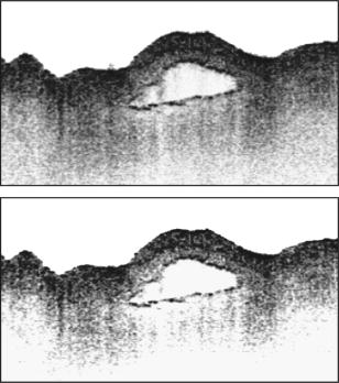

Table 1

Summary of the properties of TD-OCT, SD-OCT, and SS-OCT.

	TD-OCT	FD-OCT	SS-OCT
Classical noise	1. $1 ∕ f$ noise, dark current noise, Johnson noise, preamplifier noise	1. $1 ∕ f$ noise, dark current noise, Johnson noise, preamplifier noise	1. $1 ∕ f$ noise, dark current noise, Johnson noise, preamplifier noise
	2. photon excess noise	2. photon excess noise	2. dc signal
	3. dc signal	3. dc signal	3. Nonlinear frequency tuning
	4. Microvibration and nonlinear motion	4. Noise unique to CCD
Mechanism to compensate for classical noise	1. Bandpass filter	1. Poorly compensate for as the system is a low-pass filter	1. Low-pass filter but can be partially compensated for by $z_{0}$ offset. High source intensity across the bandwidth, and fast sweep rate.
	2. Dual balanced detection	2. Time integration gives some improvement but limited by motion artifacts
	3. Algorithms if micro-vibration is significant	3. $z_{0}$ offset can give some improvement but lead to modulation depth distortion
		4. EO phase modulation proposed but lead to issues analogous to mechanical translation
		5. Photon excess noise not easily compensate for
CCD		1. Read noise and reset noise
		2. Increased classical noise
		3. Time integration restricted by sample motion artifacts
AD converter’s dynamic range	1. $\log_{10}$ demodulation allows dynamic range approaching $80 dB$ .	1. The use of digital Fourier transform prevents $\log_{10}$ demodulation. Dynamic range of $40 dB$	1. Same as FD-OCT.
Quantum noise	1. Photon shot noise, radiation pressure vacuum fluctuations, and current shot noise. The first three has same magnitude to FD-OCT but less than SS-OCT.	1. Same as TD-OCT.	1. Photo shot noise, radiation pressure and vacuum fluctuation greater than TD-OCT and FD-OCT.
Conclusion	1. Through bandpass filter, dual balanced detection, and control of motion nonlinearity, SNR approaches quantum noise limit.	1. Low-pass filter allows high classical noise.	1. Low-pass filter allows high classical noise
	2. Dynamic range approaching $80 dB$ .	2. Dual balanced detector not possible to remove excess noise.	2. Low excess noise
		3. CCD associated with unique noise sources.	3. Now limited to fast sweep rate
		4. Dynamic range approaches $40 dB$ .	4. Increased quantum noise
		5. $z_{0}$ offset, time integration and use of EO phase modulation unlikely to overcome these limitations.	5. $z_{0}$ offset, high source intensity across the bandwidth, and fast sweep rate may lead to SNR near TD-OCT
			6. Dynamic range limited to $40 dB$ .

Signal-to-noise ratio

This is the ratio of the amplitude of the maximal signal to the amplitude of noise signals at a given point in time. SNR is usually expressed in decibels and in terms of peak values for impulse noise and root-mean-square values for random noise. In defining or specifying the SNR, both the signal and noise should be characterized ( $e$ . $g$ ., peak-signal-to-peak-noise ratio) to avoid ambiguity. Photocurrent is the detected parameter in TD-OCT and SS-OCT, whereas photo-generated charge numbers are the detected parameter in FD-OCT. The different parameters do not affect the SNR if the parameters are appropriately defined. Most SNR are describing the analog or rf signal prior to digitization.

Sensitivity

In an electronic device ( $e$ . $g$ ., a communications system receiver, or detection device, $e$ . $g$ ., PIN diode), the minimum input signal required to produce a specified output signal having a specified SNR or other specified criteria is termed “sensitivity.” With OCT, the SNR is often chosen as 1. So the minimum input signal, usually defined as the minimum sample reflection intensity, equals the amount of signal that can produce the same amount of output as noise. As is discussed later, image penetration is the contrast as a function of depth, dependent more on dynamic range than sensitivity. The OCT technology is not measuring total backscattered photons but the autocorrelation.

Decibel

We define decibel as:

decibels = 10 \log x .

However, this can be confusing, since some authors use a definition found in the electronics literature:

decibels = 20 \log x .

The reasons for this are discussed elsewhere.²³ Therefore, this can result in the second yielding SNR and dynamic range value twice that of the first for the same system.

Resolution

The resolution here is defined as the full width half maximum (FWHM) of the point spread function measured from a totally reflective surface in vacuum (air for approximation.)

Contrast

There are many definitions of contrast, which are distinct from resolution. However, we use the simple definition as

\frac{I_{\max} - I_{\min}}{I_{\max} + I_{\min}},

where

I_{\max}

and

I_{\min}

represent the maximum and minimum luminance.

Penetration

In describing penetration with OCT, we are not discussing individual photon penetration but the contrast as a function of depth. Essentially, we are only at the ability to discriminate structure and not measure absolute photon counts. This is determined by the dynamic range, multiple scattering, resolution, and to a lesser degree of total power. Dynamic range is the important parameter with respect to this work. For OCT, high sensitivity allows lower photon numbers to be detected, but is not equivalent to image contrast as a function of depth.

3. Noise

We focus on three general sources of noise: those generated by the light source, the interferometer, and the detector/electronics. In some instances, sources of signal loss ( $e$ . $g$ ., AD conversion) are referred to as noise for the convenience of grouping, but the authors recognize this is a liberal use of the term.

The major light source noise contributions are photon shot noise and photon excess noise. The photon shot noise is intrinsic to the quantum nature of the source, although it can be explained qualitatively but not quantitatively from a classical approach. Generally, the sources used in OCT, super luminescent diodes (SLD), quantum well devices (below the lasing threshold), and broadband lasers follow Bose-Einstein statistics, while single-mode lasers (over the inversion threshold) follow Poisson statistics. However, at low photon counts, the primary focus of this work, the Poisson and Bose-Einstein statistics are very similar, making the distinction less than critical. There are believed to be two major sources of photon shot noise.²⁴ The first is spontaneous fluctuations (position-momentum uncertainty) at optical frequencies of electrons localized in the atomic or crystalline field of the source. The second is field fluctuations caused by the quantum-mechanical uncertainty of electric and magnetic fields. Super luminescent diodes (SLD), quantum well devices, and broadband lasers, in addition to exhibiting photon shot noise, produce photon excess noise. This is a classical noise in excess of photon shot noise and can be on the order of $19 dB$ .^{25, 26} An important source of photon excess noise is second-order correlations or photon bunching, often referred to as Brown-Twiss correlations.²⁷ Since the arrival times of bunched photons in a matched dual detector OCT system will occur almost simultaneously, this technique can be used to remove significant amounts of excess noise.²⁸ We see that dual balanced detection allows for substantial reduction of noise for TD-OCT but not for FD-OCT.²⁹ SS-OCT, which uses light that is nearly monochromatic, still may benefit from dual balanced detection.

Imbalance in power between the two arms results in reduced visibility of interference fringes. The simplest way to explain that phenomenon is to reiterate that first-order interference depends absolutely on indistinguishable paths in the two arms.³⁰ If the reference arm power is substantially greater than the sample arm, the two arms are no longer completely indistinguishable and therefore interference is reduced. This is often referred to as the Welcher Weg problem.

Within the interferometer, there are several major sources of noise that include photon pressure, the dc offset, mechanical vibrations, imbalance in power between arms, and vacuum fluctuations. Photon pressure and vacuum fluctuation will be detailed in a separate publication. Mechanical noise created by altering the path length in the reference arm is discussed under TD-OCT. A dc component is produced in the interferometer as part of the interference effect, as seen in the next section [Eq. 7]. The dc offset needs to be filtered out for the system to approach the quantum noise limit. With the low-pass filter design of SD-OCT, complete filtration of the dc offset may not be possible.

Classical electronic noise needs to be considered when comparing technologies. This includes $1 ∕ f$ noise, thermal noise (Johnson noise and dark current), and preamplifier noise. In addition, noise specific to the CCD and signal loss differences in AD conversion are discussed in subsequent sections.

At any junction, including metal-to-metal, metal-to-semiconductor, and semiconductor-to-semiconductor, conductivity fluctuations occur from $1 ∕ f$ noise. The causes of these fluctuations are still not completely understood. The standard deviation of $1 ∕ f$ noise current is given by²³:

Eq. 1

σ_{n f} \propto I_{d} {(\frac{Δ f}{f})}^{1 ∕ 2} .

The shunt resistance $R_{s h}$ in a photodiode has a Johnson or Nyquist noise associated with it. It is associated with voltage across a dissipative circuit element. These fluctuations are most often caused by the thermal motion of the charge carriers. The magnitude of this generated current noise is³¹:

Eq. 2

σ_{n T} = {(\frac{4 k T Δ f}{R_{sh}})}^{1 ∕ 2} .

Dark current, which is often confused with current shot noise, occurs in the absence of an irradiance field and follows predominately classical thermodynamic principles. It results when random electron-hole pairs are excited by sufficient thermal energy to enter the conduction band.³²

Preamplifier cascaded to the photodiode does contribute to the noise characteristics of the system. But it contributes less than the noise from the photodiode. Therefore, it is not likely to be significant with TD-OCT.

A nonclassical electronic noise source is current shot noise, which is due primarily to momentum-position uncertainty of the electrons in the current.^{24, 33} In the second quantization description, the wave function of the system is described in terms of the occupation numbers of one electron state, where the occupation numbers can take on values of 0 or 1, in accordance with the exclusion principle. The alternative is to describe the many-electron wave functions of the system as a Slater determinant of one-electron wave functions. Contrary to many misconceptions, the electron shot noise of the detector is not noise produced by photon shot noise, thermal noise, or vacuum fluctuations. A small amount of current shot noise also results from quantum mechanical tunneling ( $i . e$ ., electrons penetrating through classically impenetrable voltage barriers). These quantum noise sources are not discussed in great detail here. But at the temperatures used during most OCT experiments, classical dark noise is still in excess of that generated by tunneling, so it can be ignored.

The ultimate objective of any OCT system is to reach the nonclassical noise limit set by quantum mechanics. Therefore, an understanding of quantum noise sources as well as second-order quantization of the light field is critical.³⁴ However, due to the extensive amount of information that needs to be addressed, this will be the source of a separate publication.

4. Noise in Charge-Coupled-Devices Versus Photodiodes

Photodiodes have classical noise sources that can be suppressed more readily in the TD-OCT but not easily in SD-OCT. These include $1 ∕ f$ noise, thermal noise in resistive elements, dark noise, and preamplifier noise. The diodes also have current shot noise that cannot be suppressed by classical methods.

Noise in a CCD is typically separated here into two types of noise above those of a PIN diode; random noise and pattern noise.³⁵ Aliasing is dealt with separately. Pattern noise is a kind of spatial noise that is induced mainly by the nonuniformity of the pixels’ responsiveness, and fixed deviations of performance between pixels in the absence of illumination. Here we focus on the random noise in individual pixels and the array. Unlike random noise, pattern noise may slightly alter the form of the autocorrelation function, but not significantly the SNR and dynamic range.

The term “alias” is originally applied to the unexpected frequency/spectral components in addition to the real spectrum of a signal, which are introduced by discrete Fourier transform (DFT). According to the Nyquist sampling theorem, if the sampling frequency/rate of the signal in direct domain ( $e$ . $g$ ., in the time domain) is at least twice that of the bandwidth of the sampled signal, there would not be any alias in the transform domain ( $e$ . $g$ ., the frequency domain). Otherwise, any signal component with frequency above half of the sampling frequency will introduce alias.

Because of the reciprocity of the Fourier transform, a similar alias might happen in the direct domain ( $e$ . $g$ ., the time domain) because of the undersampling in the frequency domain.¹⁷ This applies to FD-OCT and SS-OCT, since any $A$ scans ( $z$ space) are converted from spectrum ( $k$ space). Thus there would be two possible alias sources in FD-OCT or SS-OCT. The first would be any structure in the sample far beyond the maximum $A$ -scan range that determines the sampling rate in spectrum. The distant structures in the sample will cause high frequency oscillations in the spectrum. Once these frequencies are higher than half the sampling rate, there would be signal alias in the $z$ space that mirrors the structures beyond maximum range into an $A$ scan within the range. The second source of aliasing in FD-OCT or SS-OCT, the noise in the spectrum, is more critical. This kind of noise is additive to the signal spectrum and can be treated as a type of white noise. This means there will always be high frequency components beyond half the sampling rate. After DFT, small pulses from the noise in $k$ space will inevitably occur in the $z$ space. Their intensities and positions are a random type of noise.

The photosensing element in each pixel of CCD is typically a photodiode. So any noise sources discussed before for the photodiode are present in CCD. Additional sources, in terms of a general name readout noise and rest noise, will contribute significantly in a CCD. A CCD employs an electronic network, including many capacitors and transistors for signal integration, signal transferring, and final output of the signal. This infrastructure is commonly named the readout stage in a CCD. Noise is generated in this readout portion of the CCD. Readout noise includes additional thermal noise and $1 ∕ f$ noise in the CCD. $1 ∕ f$ noise arises mainly in transistor circuits where there are numerous junctions, which implies a critical role of $1 ∕ f$ noise in the CCD. CCD employed in FD-OCT cannot suppress such a noise simply, which will deteriorate the detecting performance more in a FD-OCT than a TD-OCT.

Each photodiode in the array has to be reset through a MOSFET during the interframe period for starting the signal integration. Effectively, this is a capacitance being charged through the resistance of the MOSFET channel. The reset noise is an uncertainty about the voltage on the capacitor and can be described as the standard deviation voltage of $\sqrt k T ∕ C$ . $k$ is the Boltzmann Constant and $T$ is the absolute temperature.

Time integration is a method to improve SNR in a CCD. A detected signal $s (t)$ with the presence of additive noise $n (t)$ can be described as a random process $X (t)$ . Assuming the signal intensity is $S$ and the standard deviation of noise intensity is $σ$ , the SNR of this process will be:

Eq. 3

SNR = \frac{S}{σ} .

If we measure such random processes $N$ times, $N$ samples $x_{1} (t)$ , $x_{2} (t)$ , $\dots$ , and $x_{N} (t)$ will be obtained. The sum of these samples will be a new random process that has the signal intensity $N \times S$ , while the standard deviation of noise intensity only increases $\sqrt N$ time as $\sqrt N \times σ$ . The consequence of such a process is that the SNR is increased as:

Eq. 4

SNR = \sqrt{N} \frac{S}{σ} .

This mechanism is used in a CCD for potentially improving SNR. Based on the operating mode of the CCD, the method of addition mentioned before is realized specifically by integration. Assuming the photocurrent of each individual photodiode in the array is $I_{p}$ , the noise in standard deviation current is $σ_{n}$ . If the photocurrent of each photodiode is read out time sequentially by a multiplexer or $x - y$ addressing, it will only be equal to a single photodiode. The readout current has not been integrated, therefore the SNR is:

Eq. 5

SNR = \frac{I_{p}}{σ_{n}} .

Typically in the CCD used with OCT, the photocurrent of each photodiode is used to charge a potential well (capacitor) during a period $Δ T$ . The accumulated charge packet represents the signal and will be transferred out. The fluctuation of the charge number is noise. According to the statistics, the mean value of the charge number (signal) increases proportionally to $Δ T$ , while the standard deviation of the charge number fluctuation (noise) is only proportional to $\sqrt Δ T$ . Hence the SNR of the readout signal will be:

Eq. 6

SNR = \frac{I_{p} Δ T ∕ e}{\sqrt{σ_{n} Δ T ∕ e}},

where

e

represents the elementary charge. From Eqs. 5, 6, the SNR is obviously improved by integration. That might partially compensate the deterioration of SNR in FD-OCT, which is induced by sources described earlier. However, it should be pointed out that an additional disadvantage of performing OCT with signal integration is that any vibrations in the system during the integration period will cause distortion in detecting performance. Therefore, its applicability to moving tissue such as coronary arteries may be limited.

5. Analog-to-Digital Conversion in Spectral Domain Optical Coherence Tomography and Time Domain Optical Coherence Tomography

In the prior discussion, signal loss from analog signal to digital (AD) conversion is not taken into account. Neither is bit error. The basic component to all AD conversion is the quantizer whose output is always the closest discrete level to the analog input. Typically, the SNR ranges from 80 to $130 dB$ (the higher for TD-OCT), which refers to the analog signal. But the displayed image has a substantially reduced dynamic range due to the signal loss associated with the limitations of AD conversion. For AD conversion, the interval $Δ$ between the discrete levels is always uniform, which determines the quantization noise ( $i . e$ ., signal loss) whose standard deviation is proportional to $Δ$ . The maximum level of the quantizer is $2^{M} Δ$ , where $M$ is the bits of an AD converter. Thus the maximum image dynamic range is limited by $M$ . A 14-bit AD converter has $\sim 40 - dB$ dynamic range for SD-OCT, which, as has been pointed out, is substantially less than TD-OCT with logarithmic demodulation.

The AD conversion and its respective signal loss are different for TD-OCT and SDOCT. In TD-OCT, digital processing is applied to the analog autocorrelation $A$ scan, which allows $\log_{10}$ demodulation to maintain a high dynamic range. In a SD-OCT, digital Fourier transform is conducted to calculate the $A$ scan signal from the quantized spectral interferogram. The dynamic range of the calculated $A$ -scan signal in the SD-OCT will therefore inevitably be reduced because the logarithmic amplification of the output signal cannot be performed. Thus, logarithmic amplification corresponds to improved penetration.

The four most common sources of bit error are: 1. offset error, 2. scale error, 3. nonlinearity, and 4. nonmonotonicity. In offset error, the zero is offset by 1/2 least significant bit, (LSB), in scale error, a linear scale error is occurring that results in a fixed error from the ideal slope, nonlinearity is $\pm 1 ∕ 2$ LSB nonlinearity, and nonmonotonicity is nonmonotonic error or $> \pm 1 ∕ 2$ LSB (but other types of errors exit as described in Ref. 38).^{23, 37} While bit error is important in OCT signal errors, it is unclear that it varies significantly among the different OCT embodiments, so it is discussed further here.

6. Embodiment and Theory

6.1.

Time Domain Optical Coherence Tomography

With TD-OCT, in the reference arm a mirror is scanned, providing a low noise $A$ scan primarily through a heterodyne detection process. The light beam from the source is evenly split by a $2 \times 2$ coupler and comes through and back in the reference and the sample arm. It then recombines at one of the ports of the coupler in terms of the exit of the interferometer. The light intensity perturbation at the exit can be described as:

Eq. 7

I_{D} = I_{R} + I_{S} + \frac{1}{2} \int_{0}^{z} \int_{0}^{\infty} G (ω) p (z^{'}) p_{R} \cos {\frac{4 π ω}{c} [n_{S} (ω) z^{'} - z_{R}]} d ω} d z^{'} .

As shown in Fig. 1, the origin of coordinates

O_{S}

in the sample arm is usually set up at the sample surface. Consequently, the origin of coordinates in the reference arm

O_{R}

will be chosen at a point from where the optical group delay to the coupler matches that between

O_{S}

and the coupler in the sample arm. In Eq. 7, the function

p (z)

represents the backscattering coefficient distribution in the sample;

z

is measured from

O_{S}

. The mirror position is

z_{R}

off the

O_{R}

. Function

G (ω)

is the intensity spectrum of the light beam with variable

ω

, the optical frequency. Its integration on the total positive frequency will be the intensity

I_{0}

. Function

n_{s} (ω)

represents the refractive index of the sample, assuming no dispersion. Constant

c

is the light velocity in vacuum.

The first term in Eq. 7 corresponds to the intensity of the reflected reference beam $I_{R}$ . The second term corresponds to the total intensity of the returned sample beam $I_{S}$ , which is a dc source contributed by all the scatters. Mutual interference of all backscattering sample waves may occur, which is called the self-correlation function of scattering, or a parasitic term.^{7, 36, 38} However, this phenomena is likely to have limited relevance to system performance (TD-OCT). If no strong reflections exist in the sample, the second term can be approximated with TD-OCT to the total incoherent intensity of the returned sample beam (dc signal). Thus $I_{R}$ and $I_{S}$ can be respectively represented as a portion of $I_{0}$ :

8.

I_{R} = \frac{p_{R}^{2} I_{0}}{4},

I_{S} = \frac{I_{0}}{4} \int_{0}^{z} p^{2} (z^{'}) d z^{'},

where the coefficient

p_{R}

(0 \leq p_{R} \leq 1)

represents the variable attenuations introduced in the reference arm. The third item in Eq. 7, the interferometric term, is the actual information carrying OCT signal (ac term), in which the diagnostic information

p (z)

is encoded. As stated, the dc terms represent a noise source that requires low-pass filtration.

For time domain operation, the light intensity perturbation is converted into an electronic signal (usually the photocurrent) by either a single optical detector or a dual balanced detector approach; the latter is used to remove excess noise.

For simplification, the intensity spectrum of the light source is assumed to have a Gaussian distribution with a full-width-half-maximum (FWHM) bandwidth $Δ_{λ}$ , and assuming that the mirror in the reference scans is at a constant velocity $V_{R}$ and no polarization alterations occur. Apart from a constant that is related to the light beam size, the time sequentially generated signal can be described in terms of the convolution as:

9.

i_{D} (t) = α (I_{R} + I_{S} + \frac{I_{0}}{2} p_{R} p (\frac{V_{R} t}{n_{S} (λ_{0})}) \otimes {\cos [\frac{4 π V_{R} t}{λ_{0}}] \exp [- \frac{4 \ln 2 {(V_{R} t)}^{2}}{Δ_{l}^{2}}]}),

Δ_{l} = \frac{2 \ln 2 λ_{0}^{2}}{π Δ_{λ}},

where

α

represents the responsiveness of the detector, which is defined as the electronic signal intensity per unit light power.

Δ_{l}

represents the FWHM coherence length of light source and

λ_{0}

is the central wavelength of the light source in vacuum. The refractive index of the sample is constant as

n_{s} (λ_{0})

. Equation 9 indicates that two major parts compose the detector output, an amplitude modulation (AM) OCT signal with a certain central frequency

f_{c} = 2 V_{R} ∕ λ_{0}

and FWHM bandwidth

Δ f_{T D} = 2 V_{R} Δ_{λ} ∕ λ_{0}^{2}

, and a dc offset caused by

I_{R}

and

I_{S}

.

The use of a mechanically induced optical group delay has parameters that need to be considered to prevent signal loss. These include optical power loss, polarization effects, and dispersion effects of the reference arm. However, these can and have been readily compensated for through traditional means. Nonlinear motion and vibrations of the translation mirror are additional potential noise sources. Generally, vibrations are low frequency and can be filtered with the bandpass filter. Nonlinear motions introduce variations in the noise floor due to the fluctuations of the dc signal. If they do enter the bandpass filter, algorithms exist for their correction.³⁹ Nonlinearities are typically present and are partially corrected via modifications in wavefunction generation. In addition, some groups have placed an electro-optical modulator (EOM) in the reference arm to reduce this noise, but it introduces other noise sources.¹⁵ Any uncorrected nonlinearities are not likely to affect SNR but rather the ranging accuracy.

TD-OCT offers several advantages in approaching high signal-to-noise ratio and near quantum noise detection. First, dual balance detection offers a mechanism for removing excess noise. Second, the Doppler shift induced by the mechanical movement offers several advantages for noise reduction. These include allowing bandpass filtration to be performed that reduces interference by the dc signal offset, $1 ∕ f$ noise, and detector thermal noise. Third, the use of a single detector has noise advantages compared with a CCD, as described earlier. Fourth, signal loss from AD conversion is less for TD-OCT relative to SD-OCT. Finally, in theory, photon shot noise, photon pressure, and vacuum fluctuations should be reduced relative to SS-OCT, since the power in a given frequency at one time is lower.

It should be noted that our observations about superior TD-OCT performance are supported through two other indirect pieces of information. First, interferometry used in an attempt to detect gravitons, which is the most sensitive approach in existence, uses time domain interferometry.⁴⁰ Second, commercial SD-OCT systems operate with SNR around $100 dB$ but dynamic range below $50 dB$ .

6.2.

Spectral Domain Optical Coherence Tomography

Replacing the single detector by an optical spectrometer or using a swept/tunable laser source instead of the wideband source can obtain the spectral interferogram at the exit of the interferometer. Multiple spectral detection approaches can be used, which are categorized into different OCT operation modes in terms of common names of FD-OCT and SS-OCT. The axial detection performance of SD-OCT can be conducted on the same base of signal evolution as TD-OCT. From Eq. 7, assuming an ideal spectrum is captured by a spectrometer without any deterioration, the spectral interferogram can be written in terms of wave number $k$ :

Eq. 10

i_{D} (k) = \frac{1}{4} α (k) G (k) [p_{R}^{2} + \int_{0}^{z} p^{2} (z^{'}) d z^{'} + 2 Re (\int_{0}^{z} p (z^{'}) p_{R} \exp {j 4 π k [n_{S} (k_{0}) z^{'} - z_{R}]} d z^{'})],

where

G (k)

is the intensity spectrum of the light beam, and

α (k)

represents a spectral coefficient for conversion from light intensity to any electronic entities, e.g., current, voltage, or charge density. If

α (k)

is assumed to be the same as the responsiveness

α

in TD-OCT, applying the reverse Fourier transform to the recorded spectrum as

Eq. 11

F^{- 1} {i_{D} (k)} = \frac{α}{4} F^{- 1} {G (k)} \otimes [F^{- 1} [p_{R}^{2} + \int_{0}^{z} p^{2} (z^{'}) d z^{'}] + F^{- 1} (\int_{0}^{z} p (z^{'}) p_{R} \exp {j 4 π k [n_{S} (k) z^{'} - z_{R}]} d z^{'} + \int_{0}^{z} p (z^{'}) p_{R} \exp {- j 4 π k [n_{S} (k) z^{'} - z_{R}]} d z^{'})] .

Assuming the refractive index is constant as

n_{s} (k_{0})

,

k_{0}

is the central wave number, the third term in the right side of Eq. 11 can be further derived as

Eq. 12

F^{- 1} (\int_{0}^{z} p (z^{'}) p_{R} \exp {j 4 π k [n_{S} (k) z^{'} - z_{R}]} d z^{'} + \int_{0}^{z} p (z^{'}) p_{R} \exp {- j 4 π k [n_{S} (k) z^{'} - z_{R}] d z^{'}}) = \int_{- \infty}^{\infty} \exp (j 2 π k z^{″}) \int_{0}^{z} p (z^{'}) p_{R} \exp j 4 π k [n_{S} (k_{0}) z^{'} - z_{R}] d z^{'} d k + \int_{- \infty}^{\infty} \exp (j 2 π k z^{″}) \int_{0}^{z} p (z^{'}) p_{R} \exp - j 4 π k [n_{S} (k_{0}) z^{'} - z_{R}] d z^{'} d k = \int_{0}^{z} p (z^{'}) p_{R} \int_{- \infty}^{\infty} \exp j 2 π k [z^{″} + 2 n_{S} (k_{0}) z^{'} - 2 z_{R}] d k d z^{'} + \int_{0}^{z} p (z^{'}) p_{R} \int_{- \infty}^{\infty} \exp j 2 π k [z^{″} - 2 n_{S} (k_{0}) z^{'} + 2 z_{R}] d k d z^{'} = p_{R} \int_{0}^{z} p (z^{'}) δ [z^{″} + 2 n_{S} (k_{0}) z^{'} - 2 z_{R}] d z^{'} + p_{R} \int_{0}^{z} p (z^{'}) δ [z^{″} - 2 n_{S} (k_{0}) z^{'} + 2 z_{R}] d z^{'} = p_{R} p [\frac{- z^{″} + 2 z_{R}}{2 n_{S} (k_{0})}] \otimes δ (- z^{″} + 2 z_{R}) + p_{R} p [\frac{z^{″} + 2 z_{R}}{2 n_{S} (k_{0})}] \otimes δ (z^{″} + 2 z_{R}) .

Finally, we can get:

Eq. 13

F^{- 1} {i_{D} (k)} = \frac{α}{4} F^{- 1} {G (k)} \otimes {F^{- 1} [p_{R}^{2} + \int_{0}^{z} p^{2} (z^{'}) d z^{'}] + p_{R} p [\frac{z^{″} + 2 z_{R}}{2 n_{S} (k_{0})}] + p_{R} p (\frac{- z^{″} + 2 z_{R}}{2 n_{S} (k_{0})})} .

Both sides of Eq. 13 are the functions of a spatial variable $z^{″}$ , which is measured in free space. The right side is a convolution between a reverse Fourier transform of the spectrum of light source (wideband source or swept/tunable laser) $G (k)$ and a superposition of three elementary functions, which are included in brackets. Within the brackets, the Fourier transform of the first term is a delta function located at $z^{″} = 0$ . The last two items are symmetrical around $z^{″} = 2 z_{R}$ . The diagnostic signal $p (z)$ is actually encoded and retrievable in either one of the last two items. Equation 13 also suggests choosing $∣ z_{R} ∣$ larger than the designated imaging depth,⁷ otherwise the quasi impulse pulse at $z^{″} = 0$ would overlap with the target signal. In other words, the path length in the reference arm is approximately a few hundred microns shorter than that in the sample arm. But as shown in Eq. 10, increasing $∣ z_{R} ∣$ could cause modulation depth distortion for high frequency components in space $k$ .³⁶ This balance represents a challenge in practically implementing the technology beyond the noise limitations alluded to.

Multiple schemes could accomplish the goal of spectral interferogram detection for SD-OCT. The scanning spectrometer is probably the most intuitive choice with its easy implementation with just a dispersion component, slit, a single detector, and a set of scanning mechanics. But with this single detector approach, the bandwidth of the detecting electronics of scanning spectrometry must be the same as that in TD-OCT to get the same $A$ -scan rate. Additionally, the benefit of classical noise suppression in TD-OCT, due to the bandpass performance, would indicate its superior performance over single detector SD-OCT, since signal integration is not utilized.

A popular spectral interferogram detection approach is to us a spectrometer with a detector array. It is also called channeled spectrometry. A dispersion component is used to separate the different spectral components. The detector array captures a discrete spectrogram, described as:

14.

i_{D}^{'} (k) = i_{D} (k) {rect (\frac{k}{Δ_{k}}) [rect (\frac{k}{γ δ_{k}}) \otimes comb (\frac{k}{δ_{k}})]},

comb (\frac{k}{δ_{k}}) = \sum_{n = - \infty}^{\infty} δ (k - n δ_{k}) n = \dots, - 2, - 1, 0, 1, 2, \dots .

The items in brackets

{}

represent the discrete sampling process by the detector array in a limited spectral range, for example, the FWHM width in the

k

space

Δ_{k}

. The comb function represents the infinite impulse sampling series with the same spectral resolution

δ_{k}

. The number of detectors in the array

M

will be as

Δ_{k} ∕ δ_{k}

. The coefficient

γ

in the rectangular function is the fill factor of an individual detector that conducts spectral average over

δ_{k}

. Thus, the retrievable signal is:

15.

F^{- 1} [i_{D}^{'} (k)] = F^{- 1} [i_{D} (k)] \otimes sinc (Δ_{k} z^{″}) \otimes [sinc (γ δ_{k} z^{″}) comb (δ_{k} z^{″})],

comb (δ_{k} z^{″}) = \sum_{n = - \infty}^{\infty} δ (z^{″} - \frac{n}{δ_{k}}) n = \dots, - 2, - 1, 0, 1, 2, \dots .

Compared to Eq. 13, Eq. 15 indicates possible signal distortion in SD-OCT by the finite discrete spectrum detection, in addition to noise consideration. However, the spectrographic detection approach does eliminate the moving parts for the $A$ scan compared with TD-OCT.

For most FD-OCT, the detector array used is a CCD imager or a photodiode array that has a photogenerated-signal integration function in addition to a photoconversion function. Such a signal integration process is called an on-focal-plane signal process in an electro-optic (E-O) imaging field. How the signal integration process affects the SNR, the sensitivity, and dynamic range of a FD-OCT is important in comparing the technologies. The general principles are described in Sec. 4, and now we look specifically at its influence on FD-OCT.

6.3.

Detector Array Signal Integration

Before addressing the SNR issue, it is important to clarify how a noise $n (z)$ transfers to $k$ space. According to the Parseval theorem, the SNR can be expressed as:

Eq. 16

SNR = \frac{{[⟨ s (z) s * (z) ⟩]}^{\frac{1}{2}}}{{[⟨ n (z) n * (z) ⟩]}^{\frac{1}{2}}} = \frac{{[\int_{- \infty}^{\infty} G_{S} (k) d k]}^{\frac{1}{2}}}{{[\int_{- \infty}^{\infty} G_{N} (k) d k]}^{\frac{1}{2}}},

where

G_{S} (k)

and

G_{N} (k)

represent the power spectrum of the signal

s (z)

and the noise

n (z)

. Equation 16 indicates no SNR change by Fourier transform. From Eq. 10, assuming that

α (k)

equals one, the captured spectrum for single scatter at depth

z_{0}

is expressed as:

Eq. 17

F (k) = \frac{1}{4} G (k) {p_{R}^{2} + p^{2} + 2 p p_{R} \cos [4 π (z_{0} - z_{R}) k]} + N (k) .

The signal spectrum will be

p p_{R} G (k) ∕ \sqrt{8}

.

First we consider a simple example of using a scanning spectrometer that has a single detector. The captured spectral interferogram is time dependent with noise as:

Eq. 18

F (t) = \frac{1}{4} G (V_{k} t) [p_{R}^{2} + p^{2} + 2 p p_{R} \cos (4 π z_{0} V_{k} t)] + N (V_{k} t),

where

V_{k}

is the spectrum scan speed, assume that this detector has the same noise intensity as the one in the TD-OCT (

i . e .

, ignoring noise sources previously described). The SNR of such a FD-OCT can be expressed as:

Eq. 19

SNR = \frac{{[\frac{1}{8} \int_{0}^{\infty} p_{R}^{2} p^{2} G^{2} (k) d k]}^{\frac{1}{2}}}{σ_{n}} = \frac{{(2 \frac{p_{R}^{2} I_{0}}{4} \frac{p^{2} I_{0}}{4})}^{\frac{1}{2}}}{σ_{n}} = \frac{\sqrt{2 I_{R} I_{S}}}{σ_{n}} .

This equation tells us that the SNR over the quantum limit using scanning spectrum capturing must be very similar to TD-OCT. But again, an important difference is that the spectrum detection here is essentially a low-pass-band filter.

Commonly, a detector array is used in a FD-OCT. For the sake of comparison, we assume each detector element is the same as the one in TD-OCT. The captured spectrums are discrete and DFT is used. Previous works indicated that, after Fourier transform, the SNR will drop off by the factor $M$ if other noise sources are predominant rather than shot noise in FD-OCT (Refs. 14, 17). The reason, which led to this questionable conclusion, could be the ignoring of the energy theorem, Parseval’s theorem in DFT, as it is noticed that the discussions on the SNR issue are all based on DFT in both references. For example, Eq. 7 in Ref. 14 sums the variances of the $M$ elements as the intensity of noise in $z$ space, which corresponds to the fact that the noise intensity after DFT is multiplied $M$ fold of the one before DFT as the result of the energy theorem. However, the same multiplication was not accordingly applied to the intensity of signal shown in Eq. 6. A slightly different expression can be seen in Ref. 17, where that the noise intensity in $z$ space was $1 ∕ M$ of the one in $k$ space (represented by the noise intensity in a single detector), which is still consistent with the energy theorem if it is assumed that inverse DFT was used. However, in Eq. 4 of the paper, the intensity of signal was not reduced as $1 ∕ M$ either, according to the energy theorem.

An alternative example to understand this process correctly is if a multiplexer is used for spectrum readout. Commonly, a detector array is used in a FD-OCT. For better comparison, we assume each detector element is the same as the one in TD-OCT. If a multiplexer is used for spectrum readout, the SNR will be the same as that of a FD-OCT using a scanning spectrometer, which yields no extraordinary benefit for using such FD-OCT setups. The signal integration function in the array is the real contributor for both possible performance improvement and deterioration. A typical detector array is a CCD imager. In each element the photogenerated electrons are accumulated and stored as a packet. Differing from all setups discussed before, the interferogram detection is essentially energy detection. Hence the spectral distribution of signal $Q_{S} (k)$ is proportional to $\sqrt{2} p p_{R} G (k) Δ T_{F D}$ , with $Δ T_{F D}$ representing the integrating time. The incoherently integrated noise in each element $Q_{n}$ will be proportional to $σ_{n}^{'} \sqrt{Δ T_{F D}}$ . $σ_{n}^{'}$ represents input-referred noise magnitude, which is bigger than $σ_{n}$ , the noise present in a single element. It is important to realize that the random noise in $k$ space has the same statistics as in a single element. Thus the SNR of a FD-OCT is determined by:

Eq. 20

SNR = \frac{Q_{S}}{Q_{n}} = \frac{{(2 I_{R} I_{S} Δ T_{FD})}^{\frac{1}{2}}}{σ_{n}^{'}} .

Adapting the SNR expression of the TD-OCT into the version of energy detection, the SNR of a TD-OCT can be described as:

Eq. 21

{SNR}_{TD} = \frac{{(2 I_{R} I_{S} Δ T_{TD})}^{\frac{1}{2}}}{σ_{n}},

where

Δ T_{TD}

is the equivalent integrating time of a TD-OCT, which is the reverse of the bandwidth of the system as

Δ T_{T D} = 1 ∕ (2 Δ f_{T D})

. We assume both TD-OCT and FD-OCT has the same scanning depth. If the spectral resolution in FD-OCT is

δ k

, the equivalent scan depth

Δ z_{\max}

in TD-OCT will be as

1 ∕ (2 δ_{k})

. If the integrating time is part of the time needed for an A-scan in TD-OCT, associated with a duty coefficient

γ (0 \leq γ \leq 1)

, the equivalent scanning speed

V_{R}

is

γ Δ f_{F D} ∕ δ_{k}

,

Δ f_{F D}

is the equivalent bandwidth of the detecting electronics in a FD-OCT equaling

Δ f_{T D} = 1 ∕ (2 Δ T_{TD})

. The equivalent system bandwidth in TD-OCT and FD-OCT will be related as

Δ f_{T D} ∕ Δ f_{F D} = γ Δ_{k} ∕ δ_{k} = γ M

. Substituting them into Eqs. 20, 21, the SNR difference between FD-OCT and TD-OCT is approximated to

σ_{n} ∕ σ_{n}^{'} \sqrt{γ M}

. Consequently the sensitivity of FD-OCT will be improved

\sqrt{γ M}

times that for TD-OCT, but depending the amount of

σ_{n}^{'}

, compared to TD-OCT.

An important disadvantage to using signal integration with OCT is that any vibrations in the system during the integration period will cause distortion in the image, limiting both its use in moving tissue and the length of the integration time.

6.4.

Swept Source Optical Coherence Tomography

An alternative way to obtain a spectrogram is to use a frequency swept laser or tunable laser with just a single detector and without dispersion components, which is referred to as SS-OCT. From Eq. 10, the detected spectrogram can be described as:

Eq. 22

i_{D}^{'} (k) = \frac{1}{4} α (k) {G (k) [\exp (- \frac{k^{2}}{2 σ_{k}^{2}}) \otimes comb (\frac{k}{δ_{k}^{'}})]} [p_{R}^{2} + \int_{0}^{z} p^{2} (z^{'}) d z^{'} + 2 Re (\int_{0}^{z} p (z^{'}) P_{R} \exp {j 4 π k [n_{S} (k_{0}) z^{'} - z_{R}]} d z^{'})] .

The spectrum of the light source is described as a discrete spectral intensity distribution with a line width

σ_{k}

(standard deviation) and tuning mode-hop

δ_{k}^{'}

. So the retrieved signal can be expressed as:

Eq. 23

F^{- 1} {i_{D} (k)} = \frac{α}{4} F^{- 1} [G (k)] \otimes [\exp (- 2 σ_{k}^{2} {z^{″}}^{2}) comb (δ_{k}^{'} z^{″})] \otimes (F^{- 1} {p_{R}^{2} + \int_{0}^{z} p_{S}^{2} (z^{'}) d z^{'}} + p (\frac{z^{″} + 2 z_{R}}{2 n_{S} (k_{0})}) + p [\frac{- z^{″} + 2 z_{R}}{2 n_{S} (k_{0})}]) .

From Eq. 23, it is seen that the mode-hop will limit the

A

-scan range and the laser line width will degrade the

A

-scan profile.

In SS-OCT, as in FD-OCT, no moving parts are required for the axial scan (ignoring the tuning mechanism in the laser source). Possible sensitivity improvement is obtained through higher spectral intensity of the laser source but not by the signal integration process. Intrinsically, TD-OCT is a bandpass signal detecting system, whereas SS-OCT is a low-pass system. Although SS-OCT uses a single detector as TD-OCT does, the detection electronics have a critical difference with TD-OCT that will cause possible degradation in sensitivity compared with TD-OCT. In a swept or tunable laser source, the total intensity over the entire spectrum can be easily kept higher than a wideband light source. Thus possible SNR improvement can be gained in SS-OCT.^{41, 42, 43} Furthermore, a bandpass filter technique can be used, by shifting the region of interest (ROI) of the sample fairly far off the plane $O_{S}$ . Thus all the high frequency spectral oscillation introduced by the interested scatters will be kept, while much of the low frequency noise is filtered out. However, if the frequency spectrum is shifted too high, it can lead to modulation depth distortion.

Another theoretical advantage of SS-OCT is that, since the low frequency noise presents significantly in the range from zero to tens of kilohertz, the tuning speed of the swept source should also be high enough to shift the spectrum of the time sequentially recorded spectral interferogram higher out of that range.

In SD-OCT, the spectral interferogram of a single reflector located at $z_{0}$ off the $O_{S}$ can be expressed according to Eq. 10 as:

Eq. 24

i (k) = \frac{α}{4} G (k) {p_{R}^{2} + p^{2} + 2 p p_{R} \cos [4 π (z_{0} - z_{R}) k]},

where

z_{R}

is the mirror position off the

O_{R}

.

The theory behind the advantages of a high tuning speed is as follows. For SS-OCT, such a spectral interferogram is detected at the output of a single photodiode by uniformly sweeping the wavelength of the laser. Assuming the source sweep over a range $Δ_{k}$ in a period $Δ t$ from a starting wave number $k_{0}$ ,¹⁴ the spectral interferogram is captured as a time-sequential signal.

Eq. 25

i (t) = \frac{α}{4} G (k_{0} + \frac{Δ_{k}}{Δ t} t) {p_{R}^{2} + p^{2} + 2 p p_{R} \cos [4 π (z_{0} - z_{R}) \frac{Δ_{k}}{Δ t} t + 4 π (z_{0} - z_{R}) k_{0}]} .

This is an AM signal with dc offset. The central frequency is

Eq. 26

f_{C} = \frac{2 Δ_{k} (z_{R} - z_{0})}{Δ t} .

It is proportional to the sweeping speed

Δ_{k} ∕ Δ t

and

(z_{0} - z_{R})

. So higher sweeping speed and larger

z_{R}

can all shift the working band to higher frequency. A bandpass filter can thus be employed for

1 ∕ f

noise suppression. The lower cutoff frequency

f_{1}

and upper cutoff frequency

f_{2}

is defined by the border of the area of interest (ROI).

27.

f_{1} = \frac{2 Δ_{k} (z_{R} - z_{2})}{Δ t},

f_{2} = \frac{2 Δ_{k} (z_{R} - z_{1})}{Δ t} .

z_{1}

and

z_{2}

is defined as the nearest and far border of ROI, respectively, and follows as

Eq. 28

0 < z_{1} < z_{2} < z_{R} .

Note that, as is the case with TD-OCT, nonlinearities at fast source sweeps now need to be considered analogous to a moving mirror in the reference arm.

7. Acquisition Rate

It should be pointed out that in at least some SD-OCT approaches in the literature, while the raw data is collected at video rate, considerable postprocessing is necessary before an image is generated. Therefore, imaging is not performed in real time and data presented may be misleading. Clarifying if imaging is performed in real time ( $i . e .$ , RF data not complied and postprocessed) in nontransparent tissue with any of these modalities is necessary before claims of superior acquisition rate can be accepted.

8. Summary

The summary of the theoretical comparison of the three technologies is listed in Table 1. Several conclusions can be made after evaluating noise sources, optoelectronics, and AD conversion losses. For TD-OCT, through the use of low-pass filtration, dual balanced detection, and control of mirror nonlinearities, SNR approaching the quantum noise limit can be achieved. In addition, the ability to use $\log_{10}$ demodulation allows dynamic ranges to approach $80 dB$ , which is critical for imaging in nontransparent tissue. For FD-OCT, its low-pass filtering properties and use of CCD technology results in difficulties in eliminating classical noise. While $z_{0}$ offset, time integration, and/or the use of EO phase modulation may improve performance, it is not likely to overcome the large amount of classical noise. In addition, due to the nature of the Fourier transform process, the dynamic range will only be on the order of $40 dB$ . With SS-OCT, the system is also low pass, but several aspects of its embodiments may improve its performance. These include $z_{0}$ offset, high intensity across the bandwidth, and fast sweep rates, in addition to the ability to use dual balanced detection. However, due to the nature of the Fourier transform process, the dynamic range will only be on the order of $40 dB$ , and quantum noise is in excess of that of the other two embodiments. Low SNR and dynamic range can be tolerated in transparent tissue such as the eye, but not in highly scattering tissue, representing most of the tissue of the body. Future work is required to assess if SS-OCT can generate SNR and dynamic range on the order of TD-OCT.

Acknowledgments

This research is sponsored by the National Institutes of Health, contracts R01-AR44812 (Brezinski), R01-EB000419 (Brezinski), R01 AR46996 (Brezinski), R01- HL55686 (Brezinski), and R01-EB002638 (Brezinski).

References

1.

M. E. Brezinski, G. J. Tearney, B. E. Bouma, J. A. Izatt, M. R. Hee, E. A. Swanson, J. F. Southern, and J. G. Fujimoto, “Optical coherence tomography for optical biopsy — Properties and demonstration of vascular pathology,” Circulation, 93 (6), 1206 –1213 (1996). 0009-7322 Google Scholar

2.

G. J. Tearney, M. E. Brezinski, B. E. Bouma, S. A. Boppart, C. Pitris, J. F. Southern, and J. G. Fujimoto, “In vivo endoscopic optical biopsy with optical coherence tomography,” Science, 276 2037 –2039 (1997). https://doi.org/10.1126/science.276.5321.2037 0036-8075 Google Scholar

3.

M. E. Brezinski and J. G. Fujimoto, “Optical coherence tomography: High-resolution imaging in nontransparent tissue,” IEEE J. Sel. Top. Quantum Electron., 5 (4), 1185 –1192 (1999). https://doi.org/10.1109/2944.796345 1077-260X Google Scholar

4.

H. Yabushita, B. E. Bouma, S. L. Houser, H. T. Aretz, I. K. Jang, K. H. Schlendorf, C. R. Kauffman, M. Shishkov, D. H. Kang, E. F. Halpern, and G. J. Tearney, “Characterization of human atherosclerosis by optical coherence tomography,” Circulation, 106 (13), 1640 –1645 (2002). https://doi.org/10.1161/01.CIR.0000029927.92825.F6 0009-7322 Google Scholar

5.

S. D. Martin, N. A. Patel, S. B. Adams, M. J. Roberts, S. Plummer, D. L. Stamper, M. E. Brezinski, and J. G. Fujimoto, “New technology for assessing microstructural components of tendons and ligaments,” Int. Orthop., 27 (3), 184 –189 (2003). 0341-2695 Google Scholar

6.

D. Huang, E. A. Swanson, C. P. Lin, J. S. Schuman, W. G. Stinson, W. Chang, M. R. Hee, T. Flotte, K. Gregory, C. A. Puliafito, and J. G. Fujimoto, “Optical coherence tomography,” Science, 254 1178 –1181 (1991). https://doi.org/10.1126/science.1957169 0036-8075 Google Scholar

7.

A. F. Fercher, C. K. Hitzenberger, G. Kamp, and S. Y. Elzaiat, “Measurement of intraocular distances by backscattering spectral interferometry,” Opt. Commun., 117 (1-2), 43 –48 (1995). https://doi.org/10.1016/0030-4018(95)00119-S 0030-4018 Google Scholar

8.

M. Wojtkowski, R. Leitgeb, A. Kowalczyk, T. Bajraszewski, and A. F. Fercher, “_{In vivo} human retinal imaging by Fourier domain optical coherence tomography,” J. Biomed. Opt., 7 (3), 457 –463 (2002). https://doi.org/10.1117/1.1482379 1083-3668 Google Scholar

9.

A. Wax, C. H. Yang, and J. A. Izatt, “Fourier-domain low-coherence interferometry for light-scattering spectroscopy,” Opt. Lett., 28 (14), 1230 –1232 (2003). 0146-9592 Google Scholar

10.

S. H. Yun, G. J. Tearney, B. E. Bouma, B. H. Park, and J. F. de Boer, “High-speed spectral-domain optical coherence tomography at

1.3 μ m

wavelength,” Opt. Express, 11 (26), 3598 –3604 (2003). 1094-4087 Google Scholar

11.

R. A. Leitgeb, W. Drexler, A. Unterhuber, B. Hermann, T. Bajraszewski, T. Le, A. Stingl, and A. F. Fercher, “Ultrahigh resolution Fourier domain optical coherence tomography,” Opt. Express, 12 (10), 2156 –2165 (2004). https://doi.org/10.1364/OPEX.12.002156 1094-4087 Google Scholar

12.

N. A. Nassif, B. Cense, B. H. Park, M. C. Pierce, S. H. Yun, B. E. Bouma, G. J. Tearney, T. C. Chen, and J. F. de Boer, “In vivo high-resolution video-rate spectral-domain optical coherence tomography of the human retina and optic nerve,” Opt. Express, 12 (3), 367 –376 (2004). https://doi.org/10.1364/OPEX.12.000367 1094-4087 Google Scholar

13.

S. R. Chinn, E. A. Swanson, and J. G. Fujimoto, “Optical coherence tomography using a frequency-tunable optical source,” Opt. Lett., 22 (5), 340 –342 (1997). 0146-9592 Google Scholar

14.

M. A. Choma, M. V. Sarunic, C. H. Yang, and J. A. Izatt, “Sensitivity advantage of swept source and Fourier domain optical coherence tomography,” Opt. Express, 11 (18), 2183 –2189 (2003). 1094-4087 Google Scholar

15.

J. Zhang, J. S. Nelson, and Z. P. Chen, “Removal of a mirror image and enhancement of the signal-to-noise ratio in Fourier-domain optical coherence tomography using an electro-optic phase modulator,” Opt. Lett., 30 (2), 147 –149 (2005). https://doi.org/10.1364/OL.30.000147 0146-9592 Google Scholar

16.

P. Andretzky, M. Knauer, F. Kiesewetter, and G. Häusler, “Optical coherence tomography by spectral radar: improvement of signal-to-noise ratio,” Proc. SPIE, 3915 55 –59 (2000). 0277-786X Google Scholar

17.

R. Leitgeb, C. K. Hitzenberger, and A. F. Fercher, “Performance of Fourier domain vs. time domain optical coherence tomography,” Opt. Express, 11 (8), 889 –894 (2003). 1094-4087 Google Scholar

18.

J. F. de Boer, B. Cense, P. H. Park, M. C. Pierce, G. J. Tearney, and B. E. Bouma, “Improved signal-to-noise ratio in spectral-domain compared with time-domain optical coherence tomography,” Opt. Lett., 28 (21), 2067 –2069 (2003). 0146-9592 Google Scholar

19.

A. M. Rollins and J. A. Izatt, “Optimal Interferometer designs for optical coherence tomography,” Opt. Lett., 24 (21), 1484 –1486 (1999). 0146-9592 Google Scholar

20.

M. E. Brezinski, Quantum noise sources in OCT system, Google Scholar

21.

P. Andretzky, M. W. Lindner, J. M. Herrmann, A. Schultz, M. Konzog, F. Kiesewetter, and G. Häusler, “Optical coherence tomography by spectral radar: dynamic range estimation and in vivo measurements of skin,” Proc. SPIE, 3567 78 –87 (1999). 0277-786X Google Scholar

22.

T. Mitsui, “Dynamic range of optical reflectometry with spectral interferometry,” Jpn. J. Appl. Phys., Part 1, 38 (10), 6133 –6137 (1999). https://doi.org/10.1143/JJAP.38.6133 0021-4922 Google Scholar

23.

P. Horowitz and W. Hill, The Art of Electronics, 615 2nd ed.Cambridge University Press, Cambridge, UK (1997). Google Scholar

24.

C. H. Henry and R. F. Kazarinov, “Quantum noise in photonics,” Rev. Mod. Phys., 68 (3), 801 –853 (1996). https://doi.org/10.1103/RevModPhys.68.801 0034-6861 Google Scholar

25.

H. Hodara, “Statistics of thermal and laser radiation,” Proc. IEEE, 53 696 –704 (1965). 0018-9219 Google Scholar

26.

K. Takada, A. Himeno, and K. Yukimatsu, “Phase-noise and shot-noise limited operations of low coherence optical-time domain reflectometry,” Appl. Phys. Lett., 59 (20), 2483 –2485 (1991). https://doi.org/10.1063/1.105981 0003-6951 Google Scholar

27.

R. Hanbury-Brown and R. Q. Twiss, “Correlation between photons in two coherent beams of light,” Nature (London), 177 27 –32 (1956). https://doi.org/10.1038/177027a0 0028-0836 Google Scholar

28.

C. C. Rosa and A. G. Podoleanu, “Limitation of the achievable signal-to-noise ratio in optical coherence tomography due to mismatch of the balanced receiver,” Appl. Opt., 43 (25), 4802 –4815 (2004). https://doi.org/10.1364/AO.43.004802 0003-6935 Google Scholar

29.

A. G. Podoleanu, “Unbalanced versus balanced operation in an optical coherence tomography system,” Appl. Opt., 39 (1), 173 –182 (2000). 0003-6935 Google Scholar

30.

Z. Ficek and S. Swain, Quantum Interference and Coherence: Theory and Experiments, Springer Press, New York (2005). Google Scholar

31.

A. Yariv, Optical Electronics in Modern Communications, Oxford University Press, New York (1997). Google Scholar

32.

J. P. Gordon, H. J. Zeiger, and C. H. Townes, “The maser—new type of microwave amplifier, frequency standard, and spectrometer,” Phys. Rev., 99 1264 (1955). https://doi.org/10.1103/PhysRev.99.1264 0031-899X Google Scholar

33.

J. R. Schrieffer, Theory of Superconductivity, 1964). Google Scholar

34.

H.-A. Bachor and P. T. H. Fisk, “Quantum noise a limit in photodetection,” Appl. Phys. B, 49 291 (1989). 0721-7269 Google Scholar

35.

A. J. P. Theuwissen, Solid-State Imaging with Charge-Coupled Devices, Kluwer Academic Publishers, Boston (1995). Google Scholar

36.

M. Wojtkowski, A. Kowalczyk, R. Leitgeb, and A. F. Fercher, “Full range complex spectral optical coherence tomography technique in eye imaging,” Opt. Lett., 27 (16), 1415 –1417 (2002). 0146-9592 Google Scholar

37.

See http://www.national.com/kbase/category/Data_Conversion.html#30 Google Scholar

38.

G. Häusler and M. W. Lindner, “Coherence radar and spectral radar—New tools for dermatological diagnosis,” J. Biomed. Opt., 3 (1), 21 –31 (1998). https://doi.org/10.1117/1.429899 1083-3668 Google Scholar

39.

J. Schmitt and A. Olszak, “High-precision shape measurement by white-light interferometry with real-time scanner error correction,” Appl. Opt., 41 (28), 5943 –5950 (2002). 0003-6935 Google Scholar

40.

K. S. Thorne, “Gravitational-wave research: Current status and future prospects,” Rev. Mod. Phys., 52 (2), 285 –297 (1980). https://doi.org/10.1103/RevModPhys.52.285 0034-6861 Google Scholar

41.

R. Huber, M. Wojtkowski, and J. G. Fujimoto, “Fourier domain mode locking (FDML): A new laser operating regime and applications for optical coherence tomography,” Opt. Express, 14 (8), 3225 –3237 (2006). https://doi.org/10.1364/OE.14.003225 1094-4087 Google Scholar

42.

W. Y. Oh, S. H. Yun, B. J. Vakoc, G. J. Tearney, and B. E. Bouma, “Ultra-speed optical frequency domain imaging and applications to laser ablation monitoring,” Appl. Phys. Lett., 88 (10), 103902 (2006). https://doi.org/10.1063/1.2179125 0003-6951 Google Scholar

43.

R. Huber, D. C. Adler, and J. G. Fujimoto, “Buffered Fourier domain mode locking: unidirectional swept laser sources for optical coherence tomography imaging at 370,000 line/s,” Opt. Lett., 31 (20), 2975 –2977 (2006). https://doi.org/10.1364/OL.31.002975 0146-9592 Google Scholar

Citation Download Citation

Bin Liu and Mark E. Brezinski "Theoretical and practical considerations on detection performance of time domain, Fourier domain, and swept source optical coherence tomography," Journal of Biomedical Optics 12(4), 044007 (1 July 2007). https://doi.org/10.1117/1.2753410

Published: 1 July 2007

Access the abstract

JOURNAL ARTICLE
12 PAGES

DOWNLOAD PAPER SAVE TO MY LIBRARY

GET CITATION

CITATIONS

Cited by 97 scholarly publications and 1 patent.

Explore citations on Lens.org

RIGHTS & PERMISSIONS

Get copyright permission Get copyright permission on Copyright Marketplace

KEYWORDS

Signal to noise ratio

Optical coherence tomography

Charge-coupled devices

Signal detection

Sensors

Interference (communication)

Signal processing

1.

Introduction

Fig. 1

2.

Definitions

Dynamic range

Fig. 2

Table 1

Signal-to-noise ratio

Sensitivity

Decibel

Resolution

Contrast

Penetration

3.

Noise

Eq. 1

Eq. 2

4.

Noise in Charge-Coupled-Devices Versus Photodiodes

Eq. 3

Eq. 4

Eq. 5

Eq. 6

5.

Analog-to-Digital Conversion in Spectral Domain Optical Coherence Tomography and Time Domain Optical Coherence Tomography

6.

Embodiment and Theory

6.1.

Time Domain Optical Coherence Tomography

Eq. 7

8.

9.

6.2.

Spectral Domain Optical Coherence Tomography

Eq. 10

Eq. 11

Eq. 12

Eq. 13

14.

15.

6.3.

Detector Array Signal Integration

Eq. 16

Eq. 17

Eq. 18

Eq. 19

Eq. 20

Eq. 21

6.4.

Swept Source Optical Coherence Tomography

Eq. 22

Eq. 23

Eq. 24

Eq. 25

Eq. 26

27.

Eq. 28

7.

Acquisition Rate

8.

Summary

Acknowledgments

References

Show All Keywords

Keywords/Phrases

Search In:

Publication Years