1.

Introduction

The cell represents a complex biological system capable of generating and responding to forces in its environment. Still, there are relatively few scientific tools that are capable of acquiring information about displacements and forces at the cellular scale. Our laboratory has developed spectral domain phase microscopy (SDPM), a noninvasive, noncontact, optical technique capable of resolving nanometer-scale motions at sample surfaces in real time.¹

A potentially important cellular application for SDPM is that of cytoskeletal rheology, which refers to the study of how the cytoskeleton deforms in response to applied forces. The cytoskeleton is crucial for cell survival, playing significant roles not only in cell structure, but also in transport, locomotion, signal transduction, and gene expression.^{2, 3} The complex structure of the cytoskeleton is not completely characterized, and of the many models put forth to describe its mechanical properties, no single model is universally accepted.^{4, 5} We show SDPM to be a useful tool for monitoring the cellular response to applied forces, and fit the resulting data to several models for cytoskeletal rheology. We recognize that a generalized rheological model cannot completely account for the regionally varying and highly dynamic properties of the cytoskeleton,⁵ but such a model allows us to take a step toward a rigorous characterization of the cytoskeleton.

There are a variety of techniques for applying a controlled force to a cell: micropipette aspiration,^{6, 7, 8} compression between microplates,^{9, 10} cell poking,¹¹ atomic force microscopy,^{12, 13, 14} optical trapping,^{15, 16, 17} magnetic trapping,^{18, 19, 20, 21, 22, 23} and magnetic twisting cytometry.^{24, 25, 26, 27} These techniques can be divided into several categories. The first two techniques, as well as some optical trapping methods,¹⁶ probe global properties of the cell, while the remainder are used to obtain local information. Of the localized techniques, a second major distinction lies in specificity. When attempting to study the properties of the cytoskeleton, it is desirable to be able to isolate the response of the cytoskeleton from that of the rest of the cell. Both optical and magnetic techniques typically apply forces through microspheres attached to the cell surface. By coating these microspheres with an appropriate protein, extracellular forces can be directed to cytoskeletal filaments through integrin receptors.²⁸ We have selected a magnetic tweezer for this study because magnetic techniques allow for a broad range of forces and are capable of applying up to several nN of force to a cell.

The most common method for cell visualization used in previous studies of cytoskeletal rheology has been video microscopy. Typically, an attached bead is pulled or twisted, and image processing algorithms are used to track the displacement of the bead centroid in a lateral direction. Using SDPM, we will show the cellular response as the cell is pulled in the vertical direction, i.e., perpendicular to the image plane of the microscope.^{15, 29} Combined with light microscopy, this technique can provide access to cellular motion in three dimensions.

The rheological properties of the cytoskeleton have been modeled using simple combinations of springs and dashpots^{9, 18, 29} to characterize its viscoelastic response. This approach is intuitive, as both the structure and dynamics of the cytoskeleton are often compared to that of cross-linked polymer networks,^{30, 31} which are commonly represented by such models.³² The most basic viscoelastic model of this type is the standard linear solid,³³ or SLS, in which the elastic component of the cytoskeleton is represented by two linear springs and the viscous component is represented by a dashpot. Figure 1a shows a commonly used model for the cytoskeleton, an SLS body in series with a dashpot.¹⁸ Its time-dependent extension, $x\left(t\right)$ , under an applied force, $F$ , is given in Eq. 1 (Ref. 33), where $k_n$ and ${\eta }_n$ represent the n'th spring constant and viscous constant, respectively, and $u\left(t\right)$ is the unit step function:

Fig. 1

(a) A commonly used mechanical model for the cytoskeleton consists of a standard linear solid (SLS) body in series with a dashpot. This model represents changes within the cell as a force, $F$ , is applied to an attached magnetic bead. It produces a fast elastic and slower viscous behavior, as seen in Eq. 1. (b) These types of models can be extended to include multiple time constants by adding additional SLS bodies [Eq. 2].

Recently, the description of the cytoskeletal response to an applied force has shifted away from simple mechanical models toward power-law models.^{10, 26, 35} In these models, it is assumed that the cytoskeleton behaves like a soft glassy material. The governing equation for a power-law response is given by the function:

One ubiquitous characteristic of previous cell rheology studies is that the resulting data are highly variable.⁵ Cell displacement distributions often span several orders of magnitude,²⁰ and the extracted parameters, most notably from mechanical models, contain significant amounts of error. A great deal of this variability may stem from the fact that individual physical differences between examined cells are often overlooked. We have attempted to reduce the variation in our measurements by accounting for the physical and geometrical differences between each cell undergoing measurement. We have chosen to fit our data to three different models, namely, a single exponential, a double exponential, and a power law.

2.

Spectral Domain Phase Microscopy Theory

Optical coherence tomography (OCT) is a noncontact, noninvasive biomedical imaging technique capable of providing high-resolution $\left(1\text{to}10\mu \mathrm{m}\right)$ images of biological samples to a depth of a few millimeters.³⁷ OCT utilizes low-coherence interferometry to achieve axial sectioning of the sample. For a light source with a Gaussian spectral line shape, the axial resolution is inversely proportional to the spectral bandwidth. The most elementary OCT system takes the form of a Michelson interferometer, where source light is split into two optical paths by a beamsplitter. The sample arm path is focused onto the sample, while the reference arm path is repetitively scanned in path length using a translating mirror. Back-reflected reference and sample arm light is recombined at the beamsplitter and incident on a detector. For spectral domain implementations of OCT (known as spectral domain optical coherence tomography), the reference mirror is fixed and the recombined light is spectrally resolved using a spectrometer with a multichannel detector such as a CCD array.³⁸ The interferometric signal is manifested as sinusoidal oscillations in the measured spectrum, where the frequency of the oscillations is directly proportional to the path length difference between the reference and sample reflectors. Thus, Fourier transformation of the spectral interferometric signal results in a depth-resolved profile or A-scan. A two-dimensional (2-D) image can be built up by laterally scanning the sample arm beam.

SDPM is a functional extension of spectral domain OCT (SDOCT)^{39, 40, 41} that allows for the measurement of nanometer-scale motions within each pixel of a SDOCT image in real time.¹ The major modification in an SDPM setup from a standard SDOCT setup is the substitution of a common path interferometer for the Michelson interferometer.⁴² A common path interferometer is essentially a folded Michelson interferometer in which the reference and sample arm occupy the same optical path. In the SDPM common path interferometer, the reflection from the bottom surface of a coverslip serves as the reference reflection, and the cells above the coverslip comprise the sample.

The spectrum recorded at the multichannel detector includes an interferometric term that contains both amplitude and phase information about the sample optical field relative to the reference field. We can imagine the sample as being composed of many small reflectors of various reflectivity, each corresponding to an interface within the sample. Each of these reflectors contributes to the spectral interferometric signal as a sinusoid with position-dependent frequency. The spectral interferogram recorded at the detector for a single sample reflector is described by:

Fourier transformation of $i\left(k\right)$ gives $I\left(x\right)$ , a one-dimensional (1-D), depth-resolved, complex-valued reflectivity profile, or A-scan (Fig. 2 ). The magnitude of this function has peak values at $x=\pm 2n\Delta x$ , corresponding to the reflector position. In order to monitor small motions, SDPM tracks phase changes as a function of time for the interference between the reference and sample reflectors. The interferometric phase is a function of the entire optical path that the sample and reference light traverses. In the SDPM common path interferometer, the reference and sample arm optical paths differ only by the distance between the bottom surface of the coverslip (reference reflection) and the cell. Thus, any changes in the interferometric phase are due to changes in the sample optical path, which is attributed to motion of the surface of the cell. Since phase and displacement are linearly related, relative changes in the subresolution position of the sample reflector can be derived from sequential phase measurements as a function of time. As phase measurements are inherently relative, each subsequent phase measurement is referenced to the initial phase at time $t=0$ . Conversion between phase and displacement is accomplished using Eq. 5, which provides time-dependent displacement profiles, shown in Fig. 2, at selected depth locations within the sample. These depths are specified to within the coherence length of the source, $\Delta x$ . Thus, we are essentially monitoring average motion within each pixel of a standard SDOCT depth profile. Here, ∠ is the phase operator, and $k_o$ is the source center wave number.

Fig. 2

The SDPM system acquires depth-resolved information from a single transverse location on the sample. (a) Illustration depicting the experimental setup. (b) A-scan, or depth profile, plotted as log(magnitude) versus depth. (c) Complex valued M-scan. Both log(magnitude) and phase are plotted versus depth and time. The magnitude of the M-scan gives a series of A-scans, while the phase of the M-scan carries information about small changes in reflector position over time. (d) Phase (displacement) versus time at several depths in the sample. Stationary surfaces, such as the top and bottom of the coverslip, do not show any change in phase over time.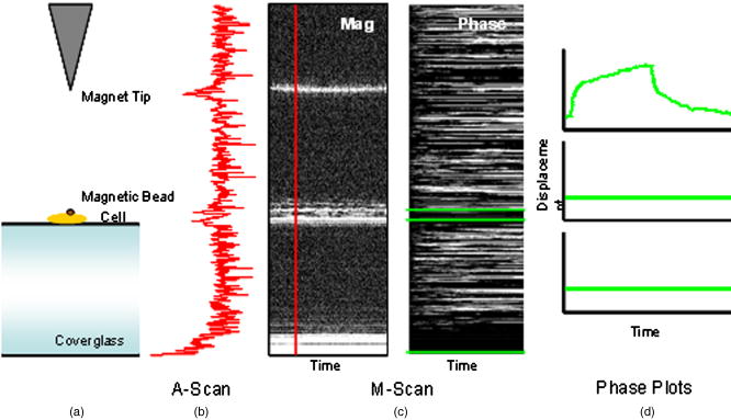

Figure 2 diagrams the information that we acquire with SDPM for the particular cellular arrangement employed in this study. We obtain a complex valued M-scan (depth profile over time) after acquiring and Fourier transforming raw SDPM data from a single transverse location over time. The magnitude of this M-scan gives us a standard SDOCT image built up of many A-scans, where reflections corresponding to the coverslip surface, the cell–magnetic bead interface, and the electromagnet tip can be clearly visualized. We also have access to the phase of this complex M-scan (relative to time $t=0$ ), and by selecting the depth corresponding to a reflection of interest, we extract a time-dependent displacement profile for that specific depth. Figure 2 also illustrates the fact that we do not see any phase changes from depths that correspond to stationary surfaces (i.e., the top and bottom of the coverslip).

The resolution of SDPM displacement measurements is limited by the phase stability of $I\left(x\right)$ . A common path interferometer is used to maximize the phase stability, since much of the phase noise is common-mode due to the shared sample and reference optical paths. With optimal displacement resolution that is less than a nanometer, SDPM is an ideal tool for making localized cellular measurements. The time resolution and sampling time of SDPM, defined by the integration time and readout time, respectively, of the spectrometer ( $\sim 5\mathrm{ms}$ and $\sim 45\mathrm{ms}$ in this study), allows for the visualization of the true dynamics of the cell. Last, SDPM is noncontact and fully compatible with light microscopy, potentially allowing for detection of motion in lateral as well as axial planes.

There are several advantages to detecting motion in an axial direction. Cells growing on a coverslip surface live in a 2-D environment, implying that cytoskeletal filments should be arranged anisotropically. It is interesting and useful to compare rheological data acquired in orthogonal directions. Additionally, since SDPM is both noncontact and noninvasive, it can potentially be used for monitoring cellular motions in three-dimensional (3-D) growth scaffolds.

We note that several other methods have been developed for monitoring cellular motions in the axial direction. Particle tracking techniques allow for the measurement of the mean square displacement (MSD) of fluorescent particles in three dimensions using tools such as cylindrical detection optics⁴³ or two-photon microscopy.^{44, 45} The MSD of particles in solutions such as cytoplasm can be used to make measurements of viscosity, as well as diffusion constants.^{43, 44} The advantage of SDPM in comparison to fluorescence-based tracking methods is that we do not need to add exogenous particles, such as fluorescent beads or other markers, to track motions of the cell. (The beads used in this study serve purely for force application.) We have demonstrated SDPM to be capable of monitoring movements of the interface defined by the top surface of the cell.¹

With respect to other magnetic microrheometers, our force application setup is quite similar to studies such as Bausch, ¹⁸ Alenghat, ²⁰ and Feneberg ²² We are capable of applying forces in the range of 100's of pN to 10's of nN in a single direction using an electromagnet milled to a sharp point. More sophisticated magnetic systems have been developed for force application in multiple directions allowing for oscillatory forces,^{19, 21} created by placing electromagnet coils on alternate sides of the cell. The advantage of our system lies in displacement data retrieval. We are capable of high-speed measurements limited by the readout time of the CCD ( $45\mathrm{ms}$ in this study), which can be as fast as sub ms (Ref. 46). Our current system speed is comparable to many of the reported magnetic microrheometers,^{18, 19} although there are both faster²⁶ and slower^{23, 29} systems as well. Additionally, our phase processing is relatively simple. We do not require particle tracking algorithms to follow the motion of the magnetic beads, as is required for many lateral tracking microrheometers.

It is illustrative to make a comparison between SDPM and other commonly used interferometric techniques. Here we will focus on reflection interference contrast microscopy (RICM), an interferometric method used to extract nanometer-scale topographical information in the one to few micron range.^{47, 48, 49, 50} RICM images are typically formed from interfering reflections of monochromatic light from the top surface of a substrate with that from the bottom surface of the target sample, allowing for a surface profile of the sample to be reconstructed. This method has been useful in applications involving the measurement of ultrathin layers,^{47, 48} as well as in investigating membrane-substrate interactions⁴⁹ and wetting phenomena.⁴⁷ RICM is capable of determining the distance between adjacent optical interfaces, as long as they correspond to the dominant reflections in the sample. By using broadband light and taking advantage of the coherence gating properties of OCT, SDPM is capable of determining relative nanometer-scale motions of multiple sample reflectors, as long as they are separated by the coherence length of the light source, on the order of several microns. This feature is particularly useful for characterizing multiple reflections, such as the cell surface and electromagnet tip reflections utilized in this study. Additionally, the sensitive spectral detection employed by SDPM allows for imaging up to several millimeters in depth.

3.

Materials and Methods

3.2.

Electromagnet Construction and Calibration

In order to apply a controlled force to the cell, an electromagnet was designed and constructed consisting of a Mu Metal core (Ed Fagan, Inc., Franklin Lakes, New Jersey), measuring $4\mathrm{cm}$ in length and $0.5\mathrm{cm}$ in diameter. The final centimeter was machined to a sharp point (Fig. 3 ). The core was wrapped with 2500 turns of $0.1\text{-}\mathrm{mm}$ copper wire. The magnet was powered by a DC power supply and mounted on a micromanipulator for translation in three dimensions. The time constant of the electromagnet was determined to be $56\mu \mathrm{s}$ . Force calibration was performed by using the electromagnet to drag the magnetic beads through a fluid of known viscosity,¹⁹ in this case, glycerol. The results can be seen in Fig. 4 for a coil current of $0.05\mathrm{A}$ . A CCD camera was used to record the motion of the beads as they traveled toward the magnet, and the velocity of a single bead was determined from its position as a function of time. Velocity is related to force through Stoke’s law for low Reynold’s number (Ref. 19), $F=3\pi \eta Dv$ , where $\eta$ is viscosity $({\eta }_{\text{glycerol}}=1500\mathrm{cP})$ , $D$ is bead diameter, and $v$ is velocity. During cell experiments, this curve was used to position the electromagnet to achieve the desired force on the magnetic bead. We chose a force of $500\mathrm{pN}$ , on the relatively flat portion of the curve, so that any error in magnet placement would cause only slight changes in the applied force.

Fig. 3

(a) Experimental setup showing the electromagnet mounted above the cell sample. The tip of the magnet was within the media during actual experiments. (b) Electromagnet schematic. (c) Photomicrograph of an MCF-7 cell with fibronectin-coated magnetic bead attached.

Fig. 4

Force calibration results for a coil current of 0.05 A. This analysis allows for the electromagnet to be appropriately positioned to deliver the desired force to the cell. We specifically chose this current to place our desired force, $500\mathrm{pN}$ , on the flat portion of the curve to prevent slight variations in magnet position from introducing a significant amount of error in the applied force. This force was not achievable in previous studies using laser tweezers.^{15, 16, 17}

3.3.

Optical Setup

The fiber-based SDPM interferometer in Fig. 5 was built using source light from a broadband femtosecond Ti:Sapphire laser (Femtolasers, Vienna, Austria), with a center wavelength of $790\mathrm{nm}$ and a $90\mathrm{nm}$ full-width half-maximum (FWHM) bandwidth. After passing through a $50∕50$ fiber coupler (AC Photonics, Santa Clara, California), SDPM light was relayed into an inverted microscope (Carl Zeiss Axiovert 200, Oberkochen, Germany) through a documentation port using lenses ${\mathrm{L}}_1$ and ${\mathrm{L}}_2$ and focused by a $20\times$ , 0.5 NA objective. The reflection from the coverslip surface closest to the interferometer served as the reference reflection. The resulting interferometric signal was detected using a commercial spectrometer (Ocean Optics USB2000, Dunedin, Florida) with a $45\mathrm{ms}$ readout rate using a $5\mathrm{ms}$ integration time. Taking advantage of the $80∕20$ beamsplitter in the microscope, it was possible to simultaneously acquire both SDPM data and visible light microscopy video, which was obtained using a CCD camera (A642, PixeLink, Ottawa, Canada) mounted on a second documentation port.

Fig. 5

SDPM common-path implementation adapted to an inverted microscope. Source light from a Ti:Sapphire laser passes through a $50∕50$ fiber coupler (FC). The beam is relayed into the microscope via a documentation port (DP). System components include the spectrometer (Spect.), collimating lens $\left({\mathrm{L}}_1\right)$ , SDPM objective lens $\left({\mathrm{L}}_2\right)$ , tube lens (TL), microscope objective $\left({\mathrm{OBJ}}_1\right)$ , coverslip (CS), camera objective $\left({\mathrm{OBJ}}_2\right)$ , and camera (CCD).

4.

Results and Discussion

The resolution of our SDPM system is determined by the interferometric phase stability at the interface of interest. The phase stability is a function of the signal-to-noise ratio (SNR) at a given point and, assuming shot noise limited detection, is determined by the source power, sample reflectivity, and integration time of the detector.¹ In the past, we have demonstrated that a similar system could operate at a stability of $22\mathrm{pm}$ using a coverslip as a test surface.¹ However, the SNR at the cell–magnetic bead interface is significantly less than that at the proximate coverslip surface due to the decreased reflectivity of this interface. We measured the average SNR of the cell–magnetic bead interface from our OCT A-scans [as shown in Fig. 2b] to be $\sim 14\mathrm{dB}$ . For this SNR, we calculated an expected phase stability of approximately $20\mathrm{nm}$ using the sensitivity expression given by Choma¹:

Representative cellular responses for both untreated and treated cells exposed to a $500\mathrm{pN}$ force are illustrated in Fig. 6 , and the average maximum cellular displacement is listed. The reported untreated cell data were averaged over 25 individual cells from a total of nine petri dishes. Treated cell data were averaged over 11 individual cells from three dishes. In each dish, the proceeding experimental procedure was performed on three to four cells, chosen at locations isolated from one another in order to reduce any residual effects from previous magnetization. Following data collection, CCD camera images of each cell were examined in order to discard those that were actually a cluster of several cells as opposed to a single cell. After $40\mathrm{s}$ of applied force, the untreated cell surfaces displaced $0.58\pm 0.34\mu \mathrm{m}$ ( $\text{mean}\pm \text{standard}$ deviation). Upon treatment with $4\mu \mathrm{M}$ Cytochalasin D, the maximum surface displacement increased dramatically to $2.40\pm 1.86\mu \mathrm{m}$ , demonstrating a decreased resistance to deformation and thus indicating that the cytoskeletal structure had been compromised. Control experiments showed that the addition of the solvent, DMSO, alone had no significant effect, as all displacements were found to be within the range defined by ± one standard deviation of the untreated responses (Fig. 6).

Fig. 6

Plot showing representative cellular responses to the application and removal of a $500\text{-}\mathrm{pN}$ force before and after $30\min$ of treatment with $4\mu \mathrm{M}$ Cytochalasin D. Average cell displacement and recovery data for 25 untreated cells and 11 treated cells is shown. A statistically significant $(\mathrm{p}<0.05)$ increase in cell displacement was seen after $30\min$ of treatment.

The individual cell response data were fit to each of the three models: the single- and double-exponential linear mechanical models [Eqs. 1, 2] as well as the power-law model [Eq. 3]. A representative cellular response fit to each of the three models can be seen in Fig. 7 . We found that the parameters associated with the double-exponential model were highly dependent on one another. Thus, the use of this model cannot be justified given the experimental data. For the remainder of this discussion, we restrict our attention to the single-exponential and power-law models. Several statistical fit parameters calculated from the nonlinear regression, including the coefficient of determination $\left({\mathrm{R}}^2\right)$ , the F statistic, the Akaike information criteria (AIC), and the predicted residual error sum of squares (PRESS) statistic, can be seen in Table 1 . These results indicated that from a statistical perspective, the single-exponential model performed better than the power-law model. The averaged extracted parameters from the two models are listed in Table 2 along with their coefficient of variation (CV), given by standard deviation/mean.

Fig. 7

A representative normal cell response fit to the (a) single-exponential [Eq. 1], (b) double-exponential [Eq. 2], and (c) power-law [Eq. 3] models. The differences in the three fits are most apparent in the first few seconds of the response. The power law model begins at zero, while both exponential models include an “instantaneous” response. All models included significant variation in the extracted parameters. Statistical goodness-of-fit metrics can be found in Table 1.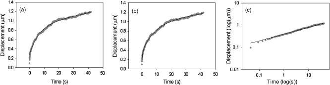

Table 1

The two models were compared based on several statistics resulting from the nonlinear regression. The coefficient of determination, or R2 , is a goodness-of-fit parameter in which values closest to 1 indicate the best fit. The X2 statistic is a measure of how close measured data points match with expected values. For both calculated X2 values, there is less than a 0.001 chance that the same results could have been obtained randomly. The F statistic is used to test the null hypothesis that all of the regression coefficients are equal to zero. Both reported F-statistics correspond to a probability of <0.0001 , allowing us to reject the null hypothesis for each model. The Akaike information criteria (AIC) is used to compare various models by selecting the best fitting model while penalizing for increasing complexity.53, 54 The absolute AIC values are unimportant; it is the difference between associated AIC values that is used to rank the models, where the smallest AIC value indicates the best model. Last, the PRESS statistic is indicative of the predictive power of the model, where the minimization of the statistic is optimal.55 Each of the statistical analysis measurements agree in ranking the single exponential better than the power law.

In order to validate our measurements with SDPM, it is necessary to compare our results to previous studies. We have presented our extracted parameters in terms of the cell surface displacement profile, $x\left(t\right)$ . Thus, our mechanical model data are in the form of spring constants, $k_n$ , and viscous constants, ${\eta }_n$ . For the purposes of comparison with previous cytoskeletal rheology studies, it is helpful to convert our measurements to elastic moduli, ${\mu }_n$ , and viscous moduli, ${\gamma }_n$ . These moduli are the constants extracted from a fit to the creep function, which is the ratio of strain to stress: $J\left(t\right)=\epsilon \left(t\right)∕{\sigma }_0=\left[x\left(t\right)A\right]∕\left[F{L}_0\right]$ , where $\epsilon \left(t\right)$ is the time-varying strain, ${\sigma }_0$ is constant stress, $A$ is area, $F$ is force, and $L_0$ is the initial thickness of the cell. Thus, we are able to back-calculate elastic and viscous moduli from our parameters using the area of the magnetic bead, $5.06\pi \mu {\mathrm{m}}^2$ , and the cell thickness. Based on separate measurements from SDPM A-scans, we estimate the average cell thickness to be approximately $8\mu \mathrm{m}$ . Our averaged single exponential parameters thus become ${\gamma }_1=82\mathrm{kN}\bullet \mathrm{s}∕{\mathrm{m}}^2$ , ${\mu }_1=1.1\mathrm{kN}∕{\mathrm{m}}^2$ , ${\mu }_2=3.0\mathrm{kN}∕{\mathrm{m}}^2$ , and ${\gamma }_2=4.0\mathrm{kN}\bullet \mathrm{s}∕{\mathrm{m}}^2$ . Lo, ²⁹ using a similar magnetic tweezers geometry, found elastic moduli ( ${\mu }_1$ , ${\mu }_2$ ) between 0.2 and $1.3\mathrm{kN}∕{\mathrm{m}}^2$ and a viscosity $\left({\gamma }_2\right)$ of $10\mathrm{kN}\bullet \mathrm{s}∕{\mathrm{m}}^2$ , which fall in the same range as our results. However, these results may not be directly comparable to our own due to the fact that the time resolution of their measurement system was on the order of seconds. Wu ’s¹⁴ AFM measurements show an elastic modulus of $2.23\mathrm{kN}∕{\mathrm{m}}^2$ and a viscosity of $5.8\mathrm{kN}\bullet \mathrm{s}∕{\mathrm{m}}^2$ , which again are similar to our findings. Both of these studies investigated the local properties of adherent cell lines to forces applied in the normal direction.

The bulk of the literature in this field presents widely varying properties and parameters to characterize the cell, often overlooking physical and geometrical differences between examined cells. It is evident that some of this variation is due to a wide array of measurement techniques and experimental setups. However, it is very likely that the individual physical characteristics of each cell contribute to its unique response. We attempted to reduce the variation in our results by accounting for differences in the cellular cross-sectional area as well as the position of the magnetic bead upon the cell. CCD images of each of the 25 normal cells were analyzed using ImageJ to measure the cross-sectional area of the cell as visualized through the microscope. As seen in Fig. 8 , decreasing cell displacement was correlated with decreasing area. Assuming a uniform distribution of integrin receptors on the cell surface, a larger area of attachment suggests that more connections have been formed between the magnetic bead and cytoskeletal filaments that are anchored to the coverslip. Thus, there are more connected pathways to resist the force of the electromagnet. We found that the area trend is best fit by a power law with an exponent of $-1.84$ . It is interesting to note that if we consider $n$ nodes in a generalized network, graph theory predicts that the number of connections between nodes scales as $n^2$ for large $n$ . We found that the strength of the cytoskeletal network scales in a similar manner. It is this increasing number of connections to anchored surfaces that imparts strength to the cell. Using this trend along with knowledge of cell thickness, and assuming a generalized 3-D shape, such as a coin-like cylinder topped by a dome,²⁹ it would be interesting to determine whether a similar trend exists in cell volume. It is likely that a larger volume of cell material would be capable of deforming farther in the vertical direction.

Fig. 8

The cross-sectional area of the adherent cell is one geometrical factor that determines how far the cell is able to stretch in the vertical direction. The area trend is best fit by a power law with exponent $-1.84$ . Rounding to $-2$ , we were able to correct our cell displacement data by dividing by the area squared. Assuming an even distribution of integrin receptors on the cell surface, the corrected model parameters describe the response of the cell on a “per-connection” basis.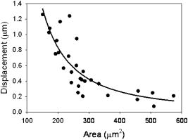

An additional parameter of potential importance is the position of the magnetic bead on the cell surface. When the microspheres were added in solution, they were observed to adhere randomly on the surfaces of the cells. It is appropriate to question whether this position affects the vertical displacement of the bead. We would expect to see more deformation near the center of the cells than near the edges, where the top and bottom surfaces of the cell are directly coupled by the actin cortex. Treating the cell images as essentially circular, a normalized radial bead position was calculated for each cell by dividing the distance from the bead to the center of the cell by the radius of the cell. Thus, a position of 1 corresponded to any edge of the cell, while 0 was the center of the cell. The average cell surface displacement of the six cells from positions between 0 and 0.3 was $0.57\pm 0.36\mu \mathrm{m}$ , and that of the eight cells from positions between 0.7 and 1.0 was $0.63\pm 0.38\mu \mathrm{m}$ . These measurements did not exhibit the anticipated trend. This discrepancy might be attributed to low sample size; we anticipate future studies measuring a larger number of cells.

The cell displacement data were corrected based on the area trend found in Fig. 8. Rounding the power-law exponent from $-1.84$ to $-2$ , we divided each displacement profile by ${\mathit{\text{area}}}^{-2}$ . By correcting for the area of the cells, we were indirectly correcting for the number of connections to the coverslip. We were, in essence, extracting new parameter values on a “per-connection” basis. This correction noticeably reduced the spread of our data, decreasing the CV in maximum cell surface displacement by 35.5%. This suggests that a portion of the large distribution of the mechanical properties of cells, observed both by ourselves and by other authors, may be due to distributions in their size and shape.

Table 2 also shows the effect of the correction on the individual parameters of each model. In each model, there are parameters that determine the final magnitude of the cellular response, $k_1$ , $k_2$ , ${\eta }_1$ , ${\eta }_2$ , and $A$ , and others that determine how quickly it reaches this final value, ${\tau }_1$ and $\alpha$ , defining the shape of the curve. We expected to see significant improvement in the parameters that govern the magnitude of displacement or stretch, but little effect upon parameters that control the time dependence of the response. The most significant improvement, a $\sim 50\%$ reduction in CV, is seen in ${\eta }_1$ , the leading dashpot in the single-exponential model. With the exception of $k_2$ , we saw the CV in all of the displacement-governing parameters decrease by 12.2% to 27.8%. Accordingly, there was very little change in the CV for ${\tau }_1$ , 0.75%. However, we still saw a relatively large improvement in the CV for $\alpha$ .

The area correction was also performed on the treated cell data in order to make a comparison between the two groups. Extracted parameters, plotted in Fig. 9 , clearly show the effects of treatment with Cytochalasin D. Again, we saw significant changes in the parameters that control the magnitude of displacement and little change in those that govern the time dependence of the curve.

Fig. 9

Comparison of averaged model parameters extracted from fits to Eqs. 1, 3 for 25 untreated and 11 drug treated cellular responses. Treated cells were exposed to a $4\text{-}\mu \mathrm{M}$ solution of Cytochalasin D for $30\min$ prior to data collection. Error bars indicate ± one standard deviation. Stars (∗) represent statistically significant differences with 95% confidence $(\mathrm{p}<0.05)$ .

Table 2

Raw model parameters extracted from nonlinear regressions to Eqs. 1, 3 were averaged over 25 untreated cellular responses and are labeled “Precorrection.” The maximum cell displacement was found to increase with decreasing cross-sectional area, prompting correction of the cell displacement data using this trend. Assuming a uniform distribution of integrin receptors on the cell surface, postcorrection parameters describe the cell behavior on a per-connection basis and reduce variation in the averaged extracted parameters. All results are reported as mean±standard deviation. The coefficient of variation (CV) is listed as a measure of cell-to-cell variation. This metric, determined as standard deviation/mean, is appropriate due to the face that precorrection and postcorrection parameters differ in units. Last, the percent reduction in the CV is listed for each parameter.

Our comparison of cytoskeletal rheology parameters before and after treatment with Cytochalasin D allows us to test predictions made by each of the postulated models. One hypothesis of previous studies that used linear mechanical models was that there should be a correlation between linear model elements and physical components of the cytoskeleton. If this were true, the drug-induced weakening of actin filaments should preferentially affect the model parameters that correspond to actin filaments and not others. However, our results indicate that the relationship is not as straightforward as a separable correlation between model parameters and physical cell components. Each spring and viscous constant in the single-exponential model appeared to be affected by drug treatment. In fact, with the exception of the leading dashpot, the decrease in each of these constants was statistically significant with $\mathrm{p}<0.05$ . These results indicate that the actin cytoskeleton contributes both an elastic and a viscous response. This finding is in agreement with Feneberg, ²² who found that the actin cortex is responsible for the viscoelastic response of the composite cell envelope.

Previous studies have used treatment with Cytochalasin D as a means of inducing a sol-gel transition.¹⁵ By weakening and dissolving actin networks, the cell should shift toward a liquid state. According to Fabry, ³⁵ the theory of soft glassy materials predicts that a phase transition occurs as the power-law exponent describing the frequency dependence of the elastic and viscous properties of the cell moves between 1 and 0. Here, an exponent of 1 describes entirely fluid-like behavior, while an exponent of 0 describes entirely solid-like behavior.³⁴ Desprat ¹⁰ found that the power-law exponents for both the frequency dependence and the time dependence of these properties are one and the same.¹⁰ If Cytochalasin D indeed moves the cell towards a sol-gel transition, we expect to see a corresponding increase in the exponent $\alpha$ . The data in Fig. 9 show a change only in the parameter $A$ , not $\alpha$ . This leads us to one of two conclusions. Either Cytochalasin D does not affect the cell in the same manner as a sol-gel transition, or soft glassy materials are not an appropriate model for the cell.

5.

Conclusions

In conclusion, we have used SDPM to monitor local nanometer-scale motions of single adherent cells under a controlled force applied through magnetic tweezers and observed the drug-induced weakening of cytoskeletal structure upon treatment with Cytochalasin D. Cell response data were fit to several cytoskeletal rheological models in order to quantitatively analyze the difference in model parameters between normal and compromised cells. We also successfully correlated the physical and geometrical properties of individual cells to displacement in order to reduce variation in our measurements. Due to its sensitivity and time resolution, SDPM appears to be a useful tool for making local measurements when studying single cell dynamics.