2.1.

Near-Infrared Tomography Simulation and Image Preparation

In previous publications, NIR frequency domain absorption and scatter tomography reconstruction has been demonstrated by several researchers, using finite element models of the diffusion approximation, and iterative reconstruction algorithms.^{17, 18, 19, 20, 21} In the work proposed in this study, the focus is on a particular experimental system design used at Dartmouth, which can produce 2-D or 3-D images of absorption and scatter coefficients of the objects examined by the noninvasive imaging array. The top level of the tomographic system detection interface is shown in Fig. 1 , with a circular arrangement of 16 linear translation stages that allow direct contact of the optical fiber bundles to the tissue being imaged. While experimental images are not used in the analysis of this study, the configuration of sources, detectors, and data noise are simulated particularly to match this experimental system, such that future studies could focus on the ROC and LROC analysis of the clinical data generated by this system.

Fig. 1

(a) A mechanical model view of the NIR imaging fiber interface is shown, using a set of 16 fiber bundles for imaging the tissue in a circular tomographic geometry, which are all moved in and out on linear translation stages, allowing imaging of different sized breasts in a circular geometry.^{5, 6} (b) Typical simulated NIR tomography images are shown with the same size and location of ROI, iteration number, and reconstruction algorithm but different contrast levels, which indicates different image quality for a typical reconstructed absorption coefficient image. At the top, the contrast was $C=1.1$ ; in the middle the contrast was $C=1.4$ , and at the bottom the contrast was $C=2.0$ .

A circular $86\text{-}\mathrm{mm}\text{-}\mathrm{diam}$ field was chosen as the background in which to place objects and test the methodology based on computed images. The finite element mesh used was a 2000 node forward 2-D geometry, which is commonly used for breast image reconstruction, which is an average spatial resolution of $1.7\mathrm{mm}$ between nodes. This field had an absorption coefficient ${\mu }_a=0.005{\mathrm{mm}}^{-1}$ , and a reduced scattering coefficient ${\mu }_s^{\prime }=1.0{\mathrm{mm}}^{-1}$ , and within this field a spherical object with fixed ${\mu }_s^{\prime }=1.0{\mathrm{mm}}^{-1}$ and a variable ${\mu }_a$ was placed to provide a localized heterogeneity. The ${\mu }_a$ value of the object was varied to simulate changes in absorption contrast, with values ranging from 1.06:1 (6%) up to to 1.3:1 (30%). The size of the object ranged from $4\text{to}16\mathrm{mm}$ in diameter. Forward calculations were based on this specific NIR tomography system geometry and diffusion theory solution using the finite element numerical method, and were used along with zero-mean Gaussian noise of 1% in amplitude and $1\mathrm{deg}$ in phase shift, to create simulated measurement data. The reconstruction algorithm was then applied to generate the 2-D absorption and scattering coefficient images. In the same manner, thousands of reconstructed images were automatically created, having the same noise level and size of heterogeneities but with different locations of the ROI and different contrasts. Similar images were created with no objects inside, to simulate normal tissue, or the “control” images. The amount and constitution of the reconstructed image pool was designed specially for several different studies presented here, and these contained images of different ROI size (4, 6, 10, and $16\mathrm{mm}$ ) or contrast, or different variations of the reconstruction algorithm, i.e., different iteration numbers of the reconstruction program or different contrast levels between the ROI and the background.

The output of the forward problem, also known as the calculated system measurement, was compared to the measured data and thereafter to determine the quality of the reconstruction process. An important measure of error in the reconstruction process is the objective function defined as:

2.2.

Human Observer Detection and Localization Tasks

Four human observers participated in this study, of which two observers had the NIR tomography imaging experience and the other two observers did not. A MATLAB program made with a graphical user interface was used as the main test program, and is shown in Fig. 2 . This controlled the data collection stage of the observer performance studies. The ROC experiment was completed by displaying a fixed number of reconstructed homogeneous or heterogeneous images in random order. After a computer-controlled training session, in which the observer was presented with sample images, then information was asked of the observed as to whether the images contained heterogeneity and also what the possible region size was. The observers were asked to view 600 different reconstructed images in one ROC experiment session. Instead of just deciding whether the viewed image was homogeneous or heterogeneous, the observers were asked to rate the probability that the image was heterogeneous, using a continuous scale value between 0 and 1, where 0 represented “absolutely homogeneous,” 1 represented “absolutely heterogeneous,” and 0.5 was a guess of “it not being known.” The observer was also asked to pick up a possible location of the ROI by selecting the centroid of the region with a mouse cursor. The observer was able to control the image contrast and brightness by adjusting the minimum and maximum display parameters of the MATLAB image profile. For every viewed image, the program recorded all of the information about this image and the decision of the observer.

Fig. 2

The image detection program is shown. Observers can adjust the image gray map scale with the top two slide bars, and point to the estimated heterogeneity location with the computer mouse.

2.3.

Computational Assessment of Contrast-to-Noise Ratio

In addition to human observer assessment, the contrast-to-noise ratio (CNR) was also used as a computational measure throughout this study. Similar to the signal-to-noise ratio in digital signal processing theory, the CNR is defined as the relative difference between the ROI and the background region values of the property, divided by the average variation in the background.^{22, 23, 24} There are different choices for the background, and here the entire region outside of the target ROI was used as the background, and thus the CNR is defined as²⁵

2.4.

Parametric and Nonparametric Receiver Operating Characteristic Analysis

ROC curves are usually generated by a model-based fit to the reader data, as illustrated in Fig. 3 . Several methods have been published to plot ROC curves based on discrete or continuous test data. These methods can be divided into two basic categories, nonparametric or parametric. The empirical nonparametric method is used to calculate the ROC curve using empirical histogram distributions, in which there is no need for structural assumptions nor parameters for model fitting. Though the empirical nonparametric method is robust and easy in some cases, it is not a smooth fitted curve leading to less conclusive analysis in the case of sparse datasets.

Fig. 3

A screen view of the graphical user interface (GUI)-based ROC fitting platform is shown, which includes empirical nonparametric initial analysis, maximum-likelihood estimation-based binormal ROC analysis, and related statistical parameter analysis such as the ROC curve confidence interval boundary, standard error, data correlation, and parameter confidence intervals.

An improvement to the empirical nonparametric method is the nonparametric kernel smoothing technique.^{13, 26, 27} In this method, a local density function, or the so-called kernel function, and a bandwidth are introduced to estimate the observer decision distribution function for diseased and healthy images. The kernel function and the bandwidth are optimized to numerically represent the distribution functions, thereby plotting a smooth and optimal ROC curve. More objective parametric methods require that some assumption be made regarding the functional form of the ROC curve. Several functional models have been proposed since ROC analysis was first developed.²⁸ One of the most popular models is the binormal ROC method, which assumes that a pair of latent normal decision variable distributions underlies the ROC data, and this has been widely used for ROC curve fitting.^{12, 29, 30, 31, 32} According to this two-parameter model, each ROC curve is assumed to have the same functional form as that implied by two Gaussian decision variable distribution functions. Within this binormal model, the task of curve fitting becomes one of choosing numerical values for the two parameter pair to best represent the measured data in observer performance studies.

The software prepared for this study includes a MATLAB command line based program, in which the empirical nonparametric approach and the maximum-likelihood estimation ROC curve fitting methods²⁹ were applied (Fig. 3). In the ROC fitting process, each image reading was assumed to be independent of all other images, thus the whole observer practice followed an independent multinomial distribution formed after classifying the continuous rating according to an ordinal classification. It was also assumed that two latent normal distributions for homogeneous and heterogeneous tissue underlie the ordinal classification, leading to a multinomial probability model for the ROC curve. Based on these two assumptions, the parameters of the ROC curve were determined via maximum-likelihood estimation ROC analysis. In the LROC fitting process, observer performance information for reconstructed images consists of two parts: 1. a continuous confidence rating of possible heterogeneity presence, and 2. coordinates representing the possible object location. The one-stage plug-in method with a biweight kernel function¹³ was used to generate the distribution bandwidth, and these were then applied to fitting the LROC curve, as illustrated in Fig. 4 . This kernel function is as described in Ref. 12, with the optimal bandwidth chosen to smooth the data. The diagnostic probability density distribution functions of normal and diseased cases are estimated to be in the form of

Fig. 4

The distributions graph of human observer responses are shown, and fitted with kernel density estimation. The window width was chosen from the direct plug-in method, and the Epanechnikov kernel was used.⁹

3.1.

Human Observer Performance Comparisons

In trying to minimize the effect of the observer’s background experience as a factor in the observer performance results, a training session was given to all participants prior to the final image presentation and detection process. In the training session, the trainee was asked to review sample images with the same reconstruction condition, and were notified if the images contained heterogeneity, and if so, what the location of the heterogeneity was. The trainee was allowed to review and analyze as many as 200 images before the real detection task began. Table 1 summarizes the area under the curve (AUC) values and associated standard error for both ROC and LROC curves for different observers in the three heterogeneity-size studies. The standard deviation between observers on the whole is less than 1% of the ROC and LROC area under the curve values, indicating that the observer performances are quite similar in this group of four subjects.

Table 1

Observer performance results for receiver operating characteristic (ROC) and location ROC (LROC) for human observers numbered 1 through 4. Note that observers 1 and 2 are experienced, and observers 3 and 4 are inexperienced.

3.2.

Human Observer Versus Computational Contrast-to-Noise Ratio Performance Comparison

3.2.1.

Heterogeneity-size study

This study was designed to evaluate how the NIR tomography imaging reconstruction algorithm response to different sized heterogeneities would affect the human perception from the images. For the sake of simplicity, a circular geometry was chosen for the heterogeneities with a diameter ranging from $4\text{to}16\mathrm{mm}$ , compared to an $86\text{-}\mathrm{mm}\text{-}\mathrm{diam}$ region for the background homogeneous tissue. Table 2 summarizes the relevant parameters of four observer performance studies, of which each study contained 600 images with optical property ranges listed in the table. To maintain experimental consistency, zero-mean Gaussian noise of 1% amplitude and $1\mathrm{deg}$ in phase shift were added to the calculated boundary data of all studies to simulate a realistic dataset from our NIR tomography system. Sample images from heterogeneity-size studies, in which objects were sized from $4\text{to}16\mathrm{mm}$ and the contrast level defined in the next section is ranged from 1.1 to 2.0, are shown in Fig. 5 .

Fig. 5

Sample images from heterogeneity-size studies are shown. The objects all have the same contrast of $C=2.0$ , the same reconstruction process iteration number $I=6$ , but with different object sizes. In (a), a small-sized object was used, with diameter of $6\mathrm{mm}$ . In (b), a medium-sized object was used, with diameter of $10\mathrm{mm}$ . In (c), a large object of diameter $16\mathrm{mm}$ was used.

Table 2

Parameter settings used in the study of heterogeneity size (iteration number=6 ).

Study	Noise level(random normallydistributed)	Heterogeneity properties		Background properties
		μa (mm−1)	Diameter(mm)	μa (mm−1)
1	1% amplitude and $1\text{-}\mathrm{deg}$ phase shift	0.0055 to 0.01	4	0.0050
2	1% amplitude and $1\text{-}\mathrm{deg}$ phase shift	0.0055 to 0.01	6	0.0050
3	1% amplitude and $1\text{-}\mathrm{deg}$ phase shift	0.0055 to 0.01	10	0.0050
4	1% amplitude and $1\text{-}\mathrm{deg}$ phase shift	0.0055 to 0.01	16	0.0050

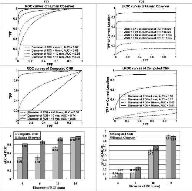
Figure 6 summarizes the human observer and computed CNR performance in the heterogeneity-size studies. In Fig. 6a, as the diameter of the target decreases down to $6\mathrm{mm}$ , the CNR value decreases below a level from which the heterogeneity can be efficiently detected, corresponding to when the AUC of the ROC is equal to 0.5. However, human observer detection is sufficiently high (above 0.5) for all heterogeneous images, even below $6\mathrm{mm}$ , having AUC values of 0.82 for $4\text{-}\mathrm{mm}$ objects and 0.88 for $6\text{-}\mathrm{mm}$ objects. As the size of the targets increases, the CNR values increase to allow for automated detection of objects in the image. Interestingly, as shown in Fig. 6b, the localization accuracy is considerably worse in these same sets of images, with objects smaller than $10\mathrm{mm}$ not being able to be localized accurately.

Fig. 6

The heterogeneity-size study for both human and computational observers is shown in (a) with ROC and area under curve data, and in (b) with LROC and AUC data. Both of these are shown for datasets where the absorption contrast ranged from 1.1 to 2.0, with a fixed six iterations.

3.2.2.

Heterogeneity contrast level study

The optical property contrast between the object and background was provided by the absorption coefficient difference between the heterogeneity and the background. The heterogeneity-to-background contrast was defined as

Eq. 5

$$C=\frac{{\mu }_{\mathrm{ROI}}}{{\mu }_{\text{background}}},$$

where ${\mu }_{\mathrm{ROI}}$ is the mean absorption coefficient of the node values in the target and ${\mu }_{\text{background}}$ is the mean absorption coefficient value over the variable background. Using fixed object diameter $D=10\mathrm{mm}$ and reconstruction process iteration number $I=6$ , and varied contrast ranging from 1.1 to 2.0 in steps of 0.1, resulted in 600 images in total. The same human and computational observers are used in these ten studies. An example image from $C=1.4$ , 1.7, and 2.0 is shown in Fig. 7 .

Fig. 7

Sample images from heterogeneity contrast studies are shown. The objects had the same size, with diameter of $10\mathrm{mm}$ , same reconstruction process with iteration number $I=6$ , but with different contrasts. In (a), the contrast was $C=1.4$ ; in (b), the contrast was $C=1.7$ ; and in (c), the contrast was $C=2.0$ .

Figure 8 summarizes the human observer and computed CNR performance in the heterogeneity contrast level studies for ROC detection task assessment [Fig. 8a] and LROC localization task assessment (Figure 8b). In Figure 8a, where the ROI size was fixed at $10\mathrm{mm}$ , the human observer performed quite well, even at low contrast levels, and achieved perfect detection $(\mathrm{AUC}=1.0)$ performance when the contrast level was above 1.6. The computed CNR, on the other hand, was unacceptably low for the 10 to 50% contrast range, but was sufficiently accurate above this range. Human observers have more capability to detect heterogeneities with small contrast levels, yet this difference was negligible if the heterogeneity was at higher contrast levels compared to the homogeneous background.

Fig. 8

The heterogeneity contrast study for both human and computational observers is shown, with (a) being the ROC curves and AUC, and (b) showing the LROC curves and area under curve. The diameter of the ROI was equal to $10\mathrm{mm}$ for all tests, and six iterations were used.

3.2.3.

Analysis of the reconstruction process iteration

The most dominant factors in the reconstruction process that affect image quality is the regularization parameter and the number of iterations used in their formation. In the presented work a modified Levenberg Marquardt scheme is used, in which the regularization parameter starts out at a high value relative to the normalized Hessian diagonal (near $100\times$ ), and then is systematically decreased by a factor of 3 at each successive iteration. Using this approach, the iteration number is the major factor influencing the detection of objects, and so this was studied here. The outline of the iteration study is summarized in Table 3 , where 600 images were used in total. During a single reconstruction process step, the 2-D image was first constructed and used as the input data for the forward problem.

In practice, as the iteration number increases, the objective function first decreases and then eventually reaches a lowest point, and then is increased very slowly, as shown in Fig. 9 . Here the ROI was $10\mathrm{mm}\mathrm{diam}$ and the contrast ranged from 1.1 to 2.0. The error was estimated from a number of reconstructions, and the mean error is plotted as a function of iteration number. In Fig. 9, the minimum objective function value occurs at an iteration number of 9. Theoretically, the reconstructed image parameter value should be closest to the true image value at the point where the objective function is at its lowest value, but in practice, the reconstruction iteration process also inevitably introduces some high-frequency spatial noise, so that it affects the judgment of both the human observers and the computational observer. Sample images from iteration numbers 4, 6, and 10 are shown in Fig. 10 .

Fig. 9

The mean of the projection error function of 294 heterogeneous reconstructed images is shown as the function of iteration number, using a diameter ROI of $10\mathrm{mm}$ and an absorption contrast range from 1.1 to 2.0. The error bars are the average standard deviations from all images.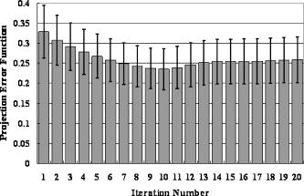

Fig. 10

Sample images from the reconstruction process are shown for different iteration numbers. The images have the same object size, $D=10\mathrm{mm}$ , the same object-to-background contrast of $C=2.0$ , but are from different numbers of iteration in the algorithm. In (a), the result from four iterations is shown. In (b), the result from six iterations is shown. And in (c), the result from ten iterations is shown.

Figure 11 summarizes the human observer and the computed CNR values for performance as a function of the iteration number for ROC detection tasks [Fig. 11a] and LROC localization tasks [Fig. 11b]. From Fig. 11, where the ROI size was fixed at $10\mathrm{mm}$ and the contrast level was varied from 1.1 to 2.0, it can be seen that the human observer always has better performance than this computed value of CNR, in terms of detectability and localization accuracy. In the range of 4 to 10 iterations, the iteration number has either negligible impact [see human observer data in Fig. 11a] or a slightly negative impact on the computed CNR data (Fig. 11) for both human observers and CNR detection and localization decisions.

Fig. 11

The reconstruction process iteration number was studied for both human and computational observers. In (a), the ROC and AUC are shown, and in (b), the LROC and AUC are shown, for a fixed diameter equal to $10\mathrm{mm}$ and with varying absorption contrast from 1.1 to 2.0.

4.1.

Assessment of the Human Observer Data

In the interhuman observer performance comparison study, AUC values for the ROC and LROC curves are summarized in Table 1. It is well known that the area under the curve of an ROC and LROC curve is a reasonable indicator of the quality of the observer performance. Given the fact that observers 1 and 2 had NIR medical experience and observers 3 and 4 were inexperienced, the main observation from Table 1 is that after the training procedure, readers without NIR imaging experience had negligible performance difference compared to readers with NIR imaging experience (i.e., less than 1% standard deviation in the AUC values overall). This trend is also observed when tested with different heterogeneity contrast levels and when the reconstruction process iteration number was varied (see Table 1). Summarizing these different tests, it was concluded that the four observers had less than 4% total variation from one another in any category of test, and the standard deviation in each test was less than 1%. These observations were important to then allow averaging of the ROC and LROC data results processed independently for all four human readers, in subsequent experimental datasets, thereby providing better power to assess the human observer results. It is always problematic to determine when averaging data from different readers is possible. However in this study all observers were given the same control of the images and all performed in a substantially similar manner, thus averaging the ROC data is a logical choice to assess the repeatability between readers. Analysis of the individual observer’s datasets were carried out, and the computed ROC AUC values did not show substantial difference from one another (less than 5% in AUC).

4.2.

Human Observer Decision Versus Computed Contrast-to-Noise Ratio

In the human observer detection process, readers were required to continuously rate the possibility of a heterogeneity being present in the images. In the computational observer detection process, the CNR value was calculated at each node and the maximum value was considered in the “decision” or “rating” of the computational observer for the NIR tomography images. Both the human observer and computational observer decision data are plotted as scatter pairs for the two image groups, including datasets where the ROI size was 10 and $16\mathrm{mm}$ . These are shown in Fig. 12 . The solid line in Fig. 12 is a linear fit of human observer and CNR values, of which the fitted equation and $R$ square value are also listed in the diagram. From Fig. 12, the main observation is that the CNR of the reconstructed images and the human observer responses are directly linearly correlated when the diameters of the targets are larger, and there is an enhanced ability of the human reader to detect smaller objects as lower CNR values. Interestingly, while the fit to the data is quite good in Fig. 12b with $R2=0.91$ , the fit to the data in Fig. 12a is not as ideal, and the shape of the data might indicate that a higher order fit is in order, perhaps with a saturation below human observer probabilities of 0.5. Further studies of this observation are ongoing, and would be consistent with the need for more complex models of human observers that require spatial matched filter analysis to accurately mimick the detection rate of a human observer.

Fig. 12

Human and computational observer performance comparisons are shown for paired sets of images analyzed. The human observer decision (confidence level that the image is abnormal) and computational observer decision (contrast-to-noise ratio) for the same group of images are plotted. A linear fitting algorithm was then applied, and the $R^2$ values are present for the two situations of (a) where contrast was set to 2.0, iterations set at six, and the object size was set at $10\mathrm{mm}$ . In (b), the contrast was still 2.0, iterations were the same, but the object size was increased to $16\mathrm{mm}$ diameter.

Table 3

Parameter settings used in the reconstruction process for the study of iteration numbers.

Examining Fig. 12, the data lines plotted cross the 50% point on the $x$ axis at a level near 3.0 to 3.3 in CNR. This represents the CNR value at which the human observer has a 50% probability of detecting an object present in the image, and thus represents the threshold level at which observers can detect objects. Below this CNR value, the human observer cannot be expected to detect the object, as they have an equal probability of not detecting it. This observation is used as a lower limit rule of thumb in interpreting the data.

4.3.

Analysis of Human Observer Versus Computed Contrast-to-Noise Ratio Decisions

Given NIR images with a suspicious object in them, it is clear that the human observer would perform better than a measure of CNR; however, the human ability to localize where the region is may not be as developed as the ability to determine if an object is present. When the object size is as small as $6\mathrm{mm}$ , the existence of this object will change the diffuse light image, but its impact is not significant enough to be detected from within the noise pattern of the image. Iterations beyond the fourth iteration tend to degrade the ability to find the location as well. Though the object is not big enough to be seen on the reconstructed image at the object true location, its presence generally makes the image seem noisier than the average homogeneous image. This entire image profile change is detectable by a human observer whose strategy and overall ability are more sensitive to noise appearance. As the heterogeneity size increases to $10\mathrm{mm}$ , it dominates the image sufficiently enough to be accurately found, and as a result, the human observers have adequate detection capability and localization accuracy. Interestingly, this phenomenon is not apparent for the CNR value, where the AUC value does not dramatically change from ROC to LROC plots. This latter point indicates that the use of CNR for tumor detection in NIR tomography images would only provide a good indicator at larger sizes and higher contrast values, whereas localization of the region may be similar to that of human observers.

An interesting area that requires further investigation is the choice of size for “detecting” a region with LROC analysis. In this study, the choice of detection versus nondetection of the location was based on using the physical size of the known object as a measure. If the observer chose outside this region, then it was counted as a mistake in localization. Given that NIR tomography has a Guassian blurred imaging field, the size of the region that is suitable to use for LROC could arguably be larger than the physical size of the existing region. However, since the resolution of the image varies with radial location, it is not obvious what choice of distance would be optimal for LROC analysis. The results here represent one interpretation. However, if the size was increased, it is likely that the statistics of LROC values would improve monotonically with the increase in size. A further analysis could be carried out where the LROC AUC is plotted as a function of the choice of diameter for “detection.”

The analysis here was completed on embedded inclusions where the contrast always increased relative to the background. In clinical studies, tumors always appear to have equal or larger vascularity, and thus have increases in contrast. So while the ROC analysis may be slightly different for situations where the contrast decreases relative to the background, this remains to be analyzed fully. Similarly, the noise levels were fixed in this analysis, and were chosen to be representative of the clinical instrument that is being used at our medical center. However, it should be expected that lower signal-to-noise level values would lead to degradation of the images and hence poorer performance in the ROC and LROC curves.