2.1.

Time-Resolved Diffuse Optical Tomography System

The design strategy for the current time-domain diffuse optical tomography (TD-DOT) system was to extend a previous fast scanning CWFT platform¹ through addition of time-resolved measurement capabilities. The system uses a planar transmission imaging geometry and provides dense spatial sampling with a large field-of-view and short scan times (Fig. 1 ). A pulsed source laser is raster-scanned across a “source” window and illuminates the imaging cassette. Light transmission through the imaging volume is profiled on the opposing “detector” window using a lens coupled gated image intensifier. The pulsed laser source (Becker & Hickel, BHLP-700, $780\mathrm{nm}$ , $T_p=100\mathrm{ps}$ , $1\mathrm{mW}$ ) provides a continuous train of light pulses (repetition rate $50\mathrm{MHz}$ ). For time-resolved detection, an ultrafast image intensifier (PicoStar HR-12, LaVision, ${\tau }_{gate}<300\mathrm{ps}$ ) relays time-gated images of the light levels on the detection plane to an electron multiplying charged coupled device (EMCCD; iXon 877f, Andor Technologies).

Fig. 1

Schematic of a TD-DOT system for small animal imaging: A pulsed laser source beam $(T_p=100\mathrm{ps})$ passes through the focusing lens and is steered by pair of galvanometer scanning mirrors to the source side of an imaging cassette. Light emitted from the detector plane of the imaging cassette is filtered and collected by a lens and temporally gated by a gated imaged intensifier. The temporally gated image is relayed to a CCD camera for readout. Timing between the source laser trigger signal and the gated detection is controlled by a programmable delay unit.

With the image intensifier operating in a “comb” mode, a sequence of gated transmissions accumulates on the EMCCD during each exposure burst. The pulse train is electronically shuttered on/off with switching times $<100\mu \mathrm{s}$ to control the burst duration (i.e., exposure time) for each source position. The light transmitted through the tissue volume is temporally resolved by scanning the delay time $\left(T_d\right)$ between the source laser pulse and the time-gated detection. The zero time delay, $T_d=0$ , is defined as the time delay at which the instrument response function is maximum. To obtain an instrument response function, a white sheet of paper is positioned in the imaging volume on the detector plane and a measurement set is taken. TD-DOT data sets consisted of measurements at 48 time-points ( $T_d$ from $-0.5\mathrm{ns}$ to $4.2\mathrm{ns}$ in steps of $0.1\mathrm{ns}$ ), with an image intensifier gate width of $0.4\mathrm{ns}$ for each source position. Temporally resolved scans are collected for each of 24 source positions, and data is extracted from the full CCD images for 24 detector positions symmetrically opposed to the source positions. The time-domain data are then converted from time-domain to frequency-domain using a Fourier transform for modulation frequencies of 208.3, 312.5, 416.7, 625, 833.3, and $1250\mathrm{MHz}$ . The frequency-domain data $\left({\Phi }_i\right)$ are indexed by $i$ , for a specified source position $r_{s\left(i\right)}$ , detector position $r_{d\left(i\right)}$ , and modulation frequency ${\omega }_i$ .

2.2.

Diffuse Optical Tomography Algorithms

In this section, we detail the algorithms used to reconstruct the optical properties using light collected at the excitation wavelength. The data, ${\Phi }_i$ , are inverted using a first-order perturbation solution of the frequency-domain diffusion approximation.^{17, 18} In the following paragraphs, we use both the diffusion coefficient $\left(D\right(\vec{r}\left)\right)$ and the reduced scattering coefficient ${\mu }_s^{\prime }\left(\vec{r}\right)$ , which are related by the simplified expression $D\left(\vec{r}\right)=\nu ∕3{\mu }_s^{\prime }\left(\vec{r}\right)$ , where $\nu$ is the speed of light in the medium.¹⁹ The perturbation expansion separates the absorption $\left({\mu }_a\right(\vec{r}\left)\right)$ and diffusion $\left(D\right(\vec{r}\left)\right)$ coefficients into background values ( ${\mu }_{a0}$ and $D_o$ ) and spatially dependent components ( $\mathrm{\Delta }{\mu }_a\left(\vec{r}\right)$ and $\mathrm{\Delta }D\left(\vec{r}\right)$ ). A scattered field, $\mathbf{y}$ , is defined as the negative log of the ratio of ${\Phi }_i^{\mathrm{target}}$ with the phantom targets over ${\Phi }_i^{\mathrm{background}}$ with only background media, $y_i=-\log ({\Phi }_i^{\mathrm{target}}∕{\Phi }_i^{\mathrm{background}})$ . The scattered field is then modeled using a linear Rytov approximation, $\mathit{y}=\mathit{Ax}$ , where $\mathit{x}=\left[\mathrm{\Delta }{\mu }_a\right(\vec{r}\left)\mathrm{\Delta }D\right(\vec{r}){]}^T=[x_a{x}_D{]}^T$ is the optical property map, and $\mathit{A}=\left[W_a{W}_D\right]$ , where $W_a$ and $W_D$ represent the sensitivity functions for the absorption and diffusion coefficients, respectively. $W_a$ and $W_s$ are expressed in terms of Green’s functions:

Since the absorption $x_a$ and diffusion $x_D$ variables differ by orders of magnitude, preconditioning of the Jacobian matrix is necessary to reduce parameter cross talk between $x_a$ and $x_D$ .^{9, 21, 22} We precondition by normalizing the absorption and diffusion variables prior to inversion using a substitution of variables $\tilde{x}=\mathit{Lx}$ , where

The penalty term for image variance is, $\alpha \Vert Q\tilde{x}{\Vert }_2^2$ , where $\alpha$ is a regularization constant, and $Q$ is a spatially variant term where $diag\left(Q\right)=sqrt\left[diag\right({\tilde{A}}^T\tilde{A}\left)\right]+\lambda$ . Last, direct inversion of $\tilde{A}$ is accomplished using a Moore-Penrose generalized inverse. After reconstruction, we convert maps of the diffusion coefficient to maps of the reduced scattering coefficient.

2.3.

Heterogeneous Optical Properties and CW Fluorescence Tomography

To provide a context for phantom tests of our TD-DOT system, we evaluated the influence of heterogeneous optical properties on fluorescence tomography for the specific situation of small animal imaging. The distribution of effective attenuation coefficients in mice was evaluated using transmitted light measurements through mice. The TD-DOT system was reconfigured for use in the CWFT mode of operation by removing the gated image intensifier and using a continuous-wave laser diode (Hiachi, HL785G, $P_{ld}=50\mathrm{mW}$ , $785\mathrm{nm}$ ).¹ An anaesthetized mouse was positioned in the imaging cassette. Transmission measurements (at the excitation wavelength without fluorescence emission filters) at opposing source-detector pairs were obtained over a $48\mathrm{mm}\times 72\mathrm{mm}$ region with 2-mm-square spacing. To provide a consistent physical path length, the tank surrounding the mouse was filled with an optically matching solution, ${\mu }_a=0.2{\mathrm{cm}}^{-1}$ , and ${\mu }_s^{\prime }=10{\mathrm{cm}}^{-1}$ , using Intralipid, water, and India ink.

In a second set of measurements, we created tissue-simulating phantoms for fluorescence tomography that matched the variation in optical properties found in the in vivo measurements. Three plastic tubes (3.5-mm OD) were placed in a background solution ( ${\mu }_a=0.1{\mathrm{cm}}^{-1}$ and ${\mu }_s^{\prime }=10{\mathrm{cm}}^{-1}$ ). Each tube had $1\mu \mathrm{M}$ concentration of Indocyanine Green (ICG) and each tube had variable concentrations of India ink. Emission and excitation measurements were obtained by scanning the phantom using a $12\times 64$ source-detector grid with 1-mm-square spacing. Fluorescence tomography reconstructions were performed using a homogeneous tissue model following previous procedures.¹

2.4.

Evaluations of Optical Property Maps Using Tissue Simulating Phantoms

The feasibility of reconstructing absorption and scattering optical property maps using the TD-DOT system was evaluated using tissue-simulating phantoms. Tubes filled with Intralipid, water, and India ink mixture to simulate objects with increased absorption ( ${\mu }_a=0.44{\mathrm{cm}}^{-1}$ , ${\mu }_s^{\prime }=15{\mathrm{cm}}^{-1}$ ) and increased scattering ( ${\mu }_a=0.12{\mathrm{cm}}^{-1}$ , ${\mu }_s^{\prime }=40{\mathrm{cm}}^{-1}$ ) were used for this purpose. The tubes were suspended in the imaging cassette filled with tissue matching fluid ( ${\mu }_a=0.12{\mathrm{cm}}^{-1}$ , ${\mu }_s^{\prime }=15{\mathrm{cm}}^{-1}$ ) and were separated by a center-to-center distance of $2\mathrm{cm}$ . Target data (with tube phantoms) and background data (without tube phantoms) were collected using the TD-DOT system in TD mode operation (Sec. 2.1).

3.1.

The Influence of Heterogeneous Optical Properties on CW Fluorescence Tomography

The heterogeneity of the optical properties in mice is illustrated by measurements of light transmission through a mouse (Fig. 2 ). The influence of heterogeneous optical properties (Fig. 2) on fluorescence tomography reconstructions is illustrated using matching tissue phantom experiments (Fig. 3 ).

Fig. 2

Variations in the light transmitted through a mouse indicate highly heterogeneous optical properties. (a) An anaesthetized mouse was positioned in the imaging cassette, and transmission measurements were obtained at opposing source-detector pairs. (b) Map of normalized transmitted light intensity measured at the excitation wavelength. (c) A log scale plot of normalized transmitted light intensity for a listing of all the source positions shows values varying by a factor of $\sim 50$ .

Fig. 3

Tissue-simulating phantom measurements were used to evaluate the influence of heterogeneous optical properties on fluorescence tomography. (a) Three plastic tubes were imaged. Each tube had the same $1\text{-}\mathrm{\mu }\mathrm{M}$ concentration of ICG but had variable concentrations of black India ink ( $1\times$ , $5\times$ , and $10\times$ more absorption than the surrounding solution ${\mu }_a=0.1{\mathrm{cm}}^{-1}$ and ${\mu }_s^{\prime }=10{\mathrm{cm}}^{-1}$ , left, center, and right, respectively). (b) The normalized transmitted light intensity measured at opposing source-detector pairs across the three tube phantoms. The variation in the light transmission (due to variations in India ink concentration) between the three tubes is similar to that encountered in vivo (Fig. 1). (c) Fluorescence tomography reconstruction of data using a homogeneous tissue model. Images of the tubes with higher absorption incorrectly indicate less fluorophore concentration.

In Fig. 2 the transmitted light intensity varies by a factor of $\sim 50$ (brightest to darkest) across the body of a mouse. Using $T\propto \exp (-{\mu }_{eff}L)$ , where $L=1\mathrm{cm}$ , and ${\mu }_{eff}$ is the effective attenuation coefficient, a 50-fold variation in $T$ corresponds to a $\sim$ fourfold variation in ${\mu }_{eff}$ . Since ${\mu }_{eff}=(3{\mu }_a{\mu }_s^{\prime }{)}^{1∕2}$ , a $\sim$ fourfold variation in ${\mu }_{eff}$ corresponds to approximately a 16-fold change in either the absorption or the reduced scattering coefficients.

The influence of this degree of heterogeneity on fluorescence tomography reconstructions was evaluated using tissue-simulating phantoms. Three tubes had identical fluorophore concentrations ( $1\mu \mathrm{M}$ ICG) and variable amounts of India ink so that the tubes left, center, and right had absorption coefficients $1\times$ , $5\times$ , and $10\times$ the background, respectively (Fig. 3). Reconstructions using a homogeneous tissue mode produce images with values that incorrectly vary by up to a factor of 5. In such situations, in situ optical property maps are needed to correctly reconstruct fluorophore distributions.

3.2.

Evaluations of TD-DOT Optical Property Maps

Figure 4 illustrates the concept of time-resolved measurements where the pulsed laser illuminates the imaging cassette and the gated intensifier time-resolves light emitted from the opposing window. Due to scattering and absorption, the detected pulse has decreased intensity and is delayed; its dependence on source-detector separation is also illustrated. Figure 4a shows the system response function with time $t=0\mathrm{s}$ along with the response to a homogeneous medium as measured by three equally spaced detectors with increasing source-detector separation. The signal amplitude falls off exponentially with increasing source-detector separation, while the mean time-of-flight increases with distance, reflecting an increase in mean path length with increased source-detector distance. The data were converted using a Fourier transform from time-domain to frequency-domain. The signal amplitude [Fig. 4b] and phase [Fig. 4c] at three representative modulation frequencies: $312.5\mathrm{MHz}$ (blue), $625\mathrm{MHz}$ (green), and, $1250\mathrm{MHz}$ (red), are shown for the middle (12th) source and all the detectors. (Color online only).

Fig. 4

Measurement setup and conversion of time-resolved measurements to frequency domain data using Fourier transform. (a) The concept of time-domain measurement is illustrated—the input laser pulse is delayed and broadened when sampled on the detector window. Two phantom targets are placed at the center of the imaging cassette and scanned using 24 source and 24 detector positions. The signal amplitude (b) and phase (c) for three modulation frequencies, $312.5\mathrm{MHz}$ (blue, top curve for amplitude and bottom curve for phase), $625\mathrm{MHz}$ (green), and $1250\mathrm{MHz}$ (red), are calculated by Fourier transform of the time-domain measurements (data shown for the 12th source and all the detectors), phase values are relative to the phase for detector 12. (Color online only)

The utility of frequency domain data for distinguishing between absorbing and scattering objects can be observed directly in the measurement data. Two tubes with diameter $5\mathrm{mm}$ were imaged, one with increased absorption ( ${\mu }_a=0.44{\mathrm{cm}}^{-1}$ , ${\mu }_s^{\prime }=15{\mathrm{cm}}^{-1}$ ), and one with increased scattering ( ${\mu }_a=0.12{\mathrm{cm}}^{-1}$ , ${\mu }_s^{\prime }=40{\mathrm{cm}}^{-1}$ ). Differential data, $y$ , is weighted by the signal-to-noise ratio (SNR) of the light intensity measurements using a noise value proportional to the square root of the intensity. In Fig. 5 , the noise-weighted differential amplitude and phase measurements for a modulation frequency of $625\mathrm{MHz}$ are depicted as images in which each pixel represents a source-detector pair. The amplitude of the scattered wave is negative for both the scattering and absorbing objects while the phase shows an increased delay for the scattering object (lower right) and decreased delay for the absorbing object (upper left). The diagonal elements of these images, which represent opposing source-detector pair measurements, are shown in Figs. 5c and 5d for modulation frequencies from $208\mathrm{MHz}$ to $1.25\mathrm{GHz}$ . Significant contrast is evident for both the scattering and the absorbing objects for all modulation frequencies.

Fig. 5

Frequency domain data: (a) amplitude and (b) phase of the noise-weighted differential measurements using a 625-MHz modulation frequency where each pixel represents a source-detector pair. The absorbing object (upper left) has decreased amplitude and a negative phase delay, while the scattering object (lower right) has decreased amplitude with a positive phase delay. The diagonal values represent opposing source-detector pair measurements, which are shown in (c) and (d) for modulation frequencies from $208\mathrm{MHz}$ to $1.25\mathrm{GHz}$ . It can be observed that lower modulation frequencies provide better amplitude contrast while higher modulation frequencies provide better phase contrast.

Figures 6a and 6b show the peak contrast in amplitude and phase for the absorption (red) and scattering (blue) objects as a function of modulation frequency. The error bars indicate standard deviation in 10 independent measurements. The amplitude contrast for the scattering object increases, while that for the absorbing object decreases with the modulation frequency. The phase contrast, on the other hand, increases with modulation frequency for both the scattering and the absorbing object. Excellent contrast and noise are obtained for modulation frequencies up to $1\mathrm{GHz}$ . At higher frequencies, the noise begins to grow significantly.

Fig. 6

The differential contrasts in (a) amplitude and (b) phase as a function of modulation frequency. The peak values in the amplitude and phase measurements corresponding to the absorption (red) and scattering (blue) object are plotted, with error bars indicating the standard deviation in 10 independent measurements.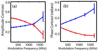

In Fig. 7 , reconstructions of the absorption (a) and scattering (b) perturbations demonstrate the capability to separate the two optical properties using data at 625-MHz modulation frequency. In order to check the quantitative accuracy of the reconstructions, we compared volume-integrated signals normalized by the phantom tube volume $V_T$ (or normalized volume integrated (NVI) signals) for the expected $NV{I}_e=\int S_{expected}\mathrm{d}v∕V_T$ and reconstructed $NV{I}_r=\int S_{reconstruction}\mathrm{d}v∕V_T$ images, where $S$ is the signal value in a voxel. The region of interest surrounding the tube phantoms is used in calculating $NV{I}_r$ . The expected values for $NV{I}_e$ are $0.32{\mathrm{cm}}^{-1}$ $\left(\mathrm{\Delta }{\mu }_a\right)$ and $25{\mathrm{cm}}^{-1}$ $\left(\mathrm{\Delta }{\mu }_s^{\prime }\right)$ . The reconstructed $NV{I}_r$ values are $0.34{\mathrm{cm}}^{-1}$ $\left(\mathrm{\Delta }{\mu }_a\right)$ and $22.58{\mathrm{cm}}^{-1}$ $\left(\mathrm{\Delta }{\mu }_s^{\prime }\right)$ , both within an error $<10\%$ with respect to the $NV{I}_e$ .

Fig. 7

(a) Frequency domain phantom data at 625-MHz modulation frequency were obtained with both an absorbing and a scattering tube (diameter $5\mathrm{mm}$ ). Reconstructed slices of (b) absorption and (c) scattering components show a clear separation of the two objects. The volume average values of contrast are in agreement with the expected values within 10% (see text).

To provide a more comprehensive evaluation, we also tested two other situations: the ability of the system to reconstruct phantoms with both absorption and scattering perturbations, and the ability to image over a range of contrasts. For the first imaging task, we reconstructed three tubes $(\mathrm{diam}=3\mathrm{mm})$ , one with only absorption contrast ( ${\mu }_a=0.44{\mathrm{cm}}^{-1}$ , ${\mu }_s^{\prime }=15{\mathrm{cm}}^{-1}$ ), one with both absorption and scattering ( ${\mu }_a=0.44{\mathrm{cm}}^{-1}$ , ${\mu }_s^{\prime }=40{\mathrm{cm}}^{-1}$ ), and one with only a scattering contrast ( ${\mu }_a=0.12{\mathrm{cm}}^{-1}$ , ${\mu }_s^{\prime }=40{\mathrm{cm}}^{-1}$ ) as shown in Figs. 8a to 8c. In the reconstructed images [Figs. 8b and 8c], each tube shows up with the appropriate combinations of contrast with minimal cross talk between absorption and scattering. For the second imaging task, we varied the absorption coefficient [Fig. 8d, ${\mu }_a=0.44{\mathrm{cm}}^{-1}$ , $0.34{\mathrm{cm}}^{-1}$ , and $0.24{\mathrm{cm}}^{-1}$ , top to bottom, respectively] while holding the reduced scattering coefficient constant and then varied the reduced scattering coefficient while holding the absorption constant [Fig. 8g, ${\mu }_s^{\prime }=20{\mathrm{cm}}^{-1}$ , $30{\mathrm{cm}}^{-1}$ , and $40{\mathrm{cm}}^{-1}$ , top to bottom, respectively]. The reconstructions performed as expected for both the absorption titration [Figs. 8e and 8f] and the reduced scattering titration [Figs. 8h and 8i]. Targets showed graded contrasts and minimal cross talk between the absorption and reduced scattering coefficients.

Fig. 8

Evaluations of mixed scattering and absorption contrast phantoms. (a) Mixed contrast targets were evaluated using three tubes (diameter $3\mathrm{mm}$ ): top tube—only ${\mu }_a$ 3.7:1; center tube—both ${\mu }_a$ 3.7:1 and ${\mu }_s^{\prime }$ 2.7:1; bottom tube— ${\mu }_s^{\prime }$ 2.7:1. All values expressed as a ratio to background optical properties ( ${\mu }_a=0.12{\mathrm{cm}}^{-1}$ , ${\mu }_s^{\prime }=15{\mathrm{cm}}^{-1}$ ). (b) Absorption coefficient reconstruction. (c) Reduced scattering coefficient reconstruction. (d) to (f) Three tubes were programmed for titrations of ${\mu }_a$ while holding ${\mu }_s^{\prime }$ fixed. (g) to (i) Three tubes were programmed for titrations of ${\mu }_s^{\prime }$ while holding ${\mu }_a$ fixed.

Using single modulation frequency measurements in the reconstruction, the interparameter cross talk is less than 10%. Similar reconstructions were obtained for 208.3, 312.5, 416.7, 833.3, and $1250\mathrm{MHz}$ modulation frequency data sets. The resolution of the scattering object [e.g., full width half maximum (FWHM)] is better than the resolution for the absorbing object at all modulation frequencies. This is in agreement with previous theoretical and experimental results.²⁴

The interaction between modulation frequency and optical properties and their combined effect on image quality for single-frequency data sets has been examined. O’Leary found in simulation studies that when background absorption is high $({\mu }_a=1{\mathrm{cm}}^{-1})$ , an increase in modulation frequency from $50\mathrm{MHz}$ to $1\mathrm{GHz}$ has no effect on image quality.¹⁷ However, for low absorption $(0.01<{\mu }_a<0.1{\mathrm{cm}}^{-1})$ , image quality improved. Jiang, ²⁵ using both simulated and measured data, found minimal effect of modulation frequency on reconstructions.

Reconstructions that combine measurements at several frequencies are expected to reduce the interparameter cross talk, provide better resolution, and increase the measurement information content. Intes ²¹ have reported simulation studies with modulation frequencies from 20 to $500\mathrm{MHz}$ where different preconditioning techniques of the weight matrix were compared for image quality and cross talk. Their results indicate that increasing the number of frequencies gave a decrease in interparameter cross talk and the column scaling preconditioning scheme resulted in less cross talk and better estimates. Gulsen ²⁶ have compared multiple-frequency reconstruction with reconstructions from various individual frequencies. Multifrequency images had lowest measurement error and highest contrast-to-noise ratio (CNR), and also the noise near the source-detector positions was reduced. Future studies with more complex phantoms and a range of object contrasts are needed to evaluate and optimize the effects of modulation frequency and multiple-frequency reconstructions for our system.