
|
|
1.IntroductionRecent technological developments have led to somewhat of a renaissance in the field of fluorescence lifetime imaging microscopy (FLIM).1 New probes and labeling techniques,2 together with new lasers, particularly for near-infrared multiphoton imaging, 3, 4, 5, 6, 7 and the introduction of inexpensive PCI card-based time-correlated single photon counting (TCSPC) boards8 has led to revived interest in time-domain microscopy. Many studies have been reported that focus on the imaging of molecular interactions9, 10 and protein conformation11, 12 in both live and fixed cells, as well as fixed human and animal sections. Despite this, some confusion persists in the analysis of data and interpretation of the results. Biexponential fits of lifetime decay curves can provide ambiguous results, with multiple combinations of parameters satisfying the conditions for a “good fit” equally well. Most frequently, cross talk can occur between the measurement of fluorescence energy transfer (FRET) efficiency, which can be used as a proxy for donor-acceptor distance and the number of interacting molecules, which is dependent on the relative amplitudes of the fluorescent decay components.13 As a result, it is frequently necessary to fix the lifetime of one or more components of the decay profile, thereby making an assumption about the homogeneity of the lifetime distribution and number of decay constants present. In addition, the presence of endogenous autofluorescence (AF) like lipofuscin14 and even photoconverted fluorophores15 can lead to a short-lived background AF. It is important to be careful in the use of control experiments to be certain that observed short lifetimes are not the result of these confounds. Other techniques have been proposed for the modeling of autofluorescence data. The use of the stretched exponential13, 16 and Laguerre deconvolution17, 18 are both powerful techniques for the inspection of tissue AF, which in of itself can yield useful information. Here, we limit ourselves to the characterization of exogenous fluorophores in the presence of AF, for the purpose of establishing FRET between interacting proteins. Although time-domain microscopy of AF can yield useful insight, for our experiments AF becomes a confound. In this study, we introduce two methods for discriminating AF signals from exogenous fluorophores in FLIM microscopy: multiple Gaussian for lifetime evaluation (MUGLE) and goodness-of-fit filtering. The fitting of experimental data to Gaussians is an approach that is widely used in science19 but has never been applied to FLIM data. Both methods take already analyzed data as input and rely on the spatial heterogeneities of the fitting parameters to better quantify results. We apply these techniques first to yellow fluorescence protein (YFP) transgenic mice that natively express YFP in a subset of cortical neurons, and extract the lifetime of YFP in the presence of background AF in the neuron. Green fluorescence protein (GFP) and its spectral variants, including YFP, have been used for applications as diverse as imaging protein interactions between fusion proteins6 and the labeling of specific organelles using targeted fusion proteins.20 The accurate determination of lifetime using FLIM in the presence of background AF opens up a myriad of possibilities to study changes in protein conformation or protein interactions in a variety of disease processes in tissue slices and eventually in intact animal. MUGLE is a general technique for characterizing and spatially segmenting lifetime distributions. As such, MUGLE has many potential applications. It could be applied whenever multiple lifetimes are present within a sample but are spatially segregated, for example in FRET experiments with samples that have heterogeneous FRET efficiencies. In a second application, we studied aged human brain samples, which are well known to contain very high levels of confounding autofluorescent substances.21 This high background has previously precluded use of FLIM-FRET approaches to the study of, for example, protein conformational changes thought to underlie human neurodegenerative diseases. We now study intracellular tau protein containing neurofibrillary tangles, which are an important pathological hallmark of Alzheimer disease (AD). While tau protein in tangles is known to be misfolded, no in-situ technique sensitive to conformation (and from specific antibodies) is available to study its tertiary structure. We apply our techniques to the study of tau pathology by double immunolabeling tau protein, to directly test a hypothesis about the conformational change that occurs when soluble tau aggregates in the cell body to form a neurofibrillary tangle. 2.Materials and Methods2.1.Yellow Fluorescence Protein Transgenic MiceTransgenic mice [B6.Cg-Tg(Thy1-YFPH)2Jrs/J] were used that express YFP in a subset of cortical neurons (Jackson Laboratory, Bar Harbor, Maine).22 Mice received an overdose of avertin ( , i.p.), then were perfused with phosphate buffered saline (PBS) followed by 4% paraformaldehyde. Brains were removed and stored in 4% paraformaldehyde/ 15% glycerol solution. Prior to use, the brain was sliced and several cortical slices were mounted with PBS on a slide. The sections were then visually inspected with wide-field microscopy to locate areas containing neurons with YFP expression that were also heavily confounded with AF. FLIM images were taken using our previously described FLIM microscope.6 All animal work conformed to National Institutes of Health (NIH) and institutional guidelines. 2.2.ImmunostainingSections of temporal lobe from Alzheimer patients [Alzheimer’s Disease Research Center (ADRC)] were immunolabeled with N-tau, an N-terminal binding antibody (1:100, courtesy of Lee, University of Pennsylvania School of Medicine, aa 2-13) and Alz50, a conformation-dependent antibody binding to N-terminal plus microtubule binding domain (MTB) (1:50; courtesy of Davies, Albert Einstein College of Medicine, aa 7-9, 312-342). N-tau was labeled with a secondary goat anti-rabbit antibody conjugated to Alexafluor 488 (A488) (1:100, Invitrogen) and Alz50 with a secondary goat anti-mouse IgM antibody conjugated to cyanine 3 (Cy3) (1:200, Jackson ImmunoResearch, West Grove, Pennsylvania). Negative controls included those labeled with donor alone and sections incubated only in blocking buffer. Positive controls made use of a tertiary donkey anti-goat antibody that place Cy3 directly apposed to A488 to ensure FRET. 2.3.Multiple Gaussian Fitting for Lifetime EvaluationThe commercial multiphoton microscope with FLIM used here has been previously described.6 FLIM images were originally analyzed using SPCImage V2.8 (Becker and Hickl GmbH). Matrices of amplitude and lifetime from either mono or biexponential fits were exported as ASCII files and postprocessed using MUGLE. The general method of fitting Gaussian curves to experimental data is widely used in many fields of science but has not been applied to FLIM, so we have included a short discussion of the principle here. In the case of multiple sources of random error of arbitrary distribution, the central limit theorem shows that the probability distribution will tend toward Gaussian,23 where represents the probability density function with respect to a given value , is the standard deviation of the distribution, and is the mean value. Considering the case where there are several discrete mean lifetimes, each with associated distributions that may overlap, a histogram of the lifetimes across all pixels would have the form,where is the intensity weighted sum of pixels of lifetime , and is half the bin width. By fitting the histogram of the intensity weighted lifetimes to this function, it is possible to recover and for distributions of multiple Gaussians. The product is proportional to the brightness of each component distribution and can therefore be used to calculate the fraction of the molecules that are responsible for a particular distribution. Further, it is possible to assign any given pixel to one particular distribution based on which is the most probable, according to the probability density functions [Eq. 1]. The resulting segmentation can be exploited to calculate the percentage of interacting molecules in the region where the lifetime of interest is observed. It is important to note that this method is dissimilar to methods like the maximum entropy method, which fits a distribution of lifetimes to a single decay curve by making use of regularization.24, 25 Instead, we fit a Gaussian to the distribution of fit results across pixels. Therefore, the size of the sample space for the Gaussian fit is the number of pixels in each sample, not the number of samples analyzed.The method of fitting was 1- minimization, where is the goodness-of-fit measure,19 using a direct Nelder-Mead26 method (Matlab function “fminsearch”). The user must input initial values for the centroid and . 2.4.Goodness-of-Fit-Based FilteringMUGLE helps separate multiple lifetime peaks that appear in the same distribution, but cannot strictly show whether the peak is due to the fluorophore or AF. To this end, a second method of eliminating AF was developed based on filtering by the goodness-of-fit parameter . Tissue AF has been shown to conform to a stretched exponential function better than a simple exponential.27 We therefore hypothesize that AF in tissue might be identifiable by higher values of than fluorescent dyes or fluorescent proteins, when tissue is fit with a mono-exponential decay. The use of the mono- rather than double-exponential decay, even for filtering samples that are expected to FRET, was used to maximize contrast between AF perturbed pixels and nonperturbed pixels. Due to the fact that multiexponential fitting is illposed in nature, a biexponential fit may well give a misleadingly low . By setting a cutoff in goodness of fit, poorly fit pixels were discarded prior to analysis. Masks were applied to the matrices of and , where the subscripts 1 and 2 refer to the shorter and longer components of the biexponential fit, and a value for percentage signal from the shorter lifetime component gives a value for the apparent fraction of interacting molecules.13 3.Results3.1.Characterization of Lifetime BroadeningTo get a sense of the variance expected from a number of pixels with the same nominal lifetime, simulated data of mono-exponential decays at values of peak photon count ranging from 1e0 to 1e5 and with , with randomly generated Poisson noise ( per level of ), was fit. The in fitted values of [Fig. 1a ] show that as signal to noise increases, the expected decreases. At an average peak count of 1e2, of would be expected if Poisson noise were the only source of error. falls to at 1e3 counts and at 1e4 counts. Fig. 1Numerical simulations to explore lifetime broadening and the separability of bi-Gaussian distributions. Simulated single exponential decay curves with added Poisson noise were fitted for a range of peak photon counts from (a) 1e1-1e5. As signal to noise increases, the lifetime broadening decreases. Experiments to empirically determine the broadening of Alexafluor 488 due to the instrument show a small but noticeable instrument broadening response, with data from ex-vivo slices with single exogenous fluorophores being broader still (not shown). Simulated data sets with a distribution such that one Gaussian was centered with zero mean and another at some separation ranging from 0 to were fit with biGaussian distributions, datasets per separation. (b) The mean and standard deviations of the fitted results show that recovery of original central values is possible when averaged over multiple samples. The uncertainty in recovered values is larger below . (c) A Kolmogorov-Smirnov (KS) analysis shows the average statistical power with respect to , at which the KS test is sensitive to the presence of multiple lifetimes for a range of type 1 error rates . On average, statistical significance (for ) would be achieved at , for data with a similar number of pixels to that obtained using our instrument.  A slide with of Alexafluor was imaged three times under the FLIM microscope. The length of time of the image acquisition was selected by trial and error to result in a range of peak counts similar those generally observed during our experiments. At an average , , at , , at , (data not shown). The interpixel variance is unsurprisingly higher than that predicted by pure Poisson noise. These data show a notable but comparatively small instrument-induced lifetime broadening. Despite the moderate interpixel broadening, the variance in lifetime between the averaged values for the three datasets is small . To give some sense of the ability of multiple Gaussian fits to distinguish between peaks in the lifetime distribution that are close together, we conducted further numerical simulations. A series of bimodal distributions (1000 randomly generated values per distribution, to match the approximate number of usable pixels in a typical FLIM experiment in our laboratory) were simulated with unit width and with the centroids being separated by a range of values between 0 and 3 standard deviations ( distributions per level of separation). The means and standard deviations [Fig. 1b] of the fitted results show good separation of the two peaks and accurate average values above , where the error bars no longer overlap. The error in the fitted peaks , above , . A Kolmogorov-Smirnov (KS) analysis shows that we can prove that a given distribution is not a monomodal Gaussian (with ) above [Fig. 1c]. Although below this level of separation of Gaussians the KS test becomes less sensitive to detecting the presence of multiple Gaussians, it is clear from Fig. 1b that we can recover Gaussians well if the separation is more than a standard deviation or so. These data taken together urge caution when analyzing overlapping peaks, although if we can be confident that two peaks do indeed exist, they can be recovered. Also, the broader error bars below suggest that for overlapping distributions, more samples may be required than for well-separated distributions to achieve specific experimental aims. 3.2.Isolation of Yellow Fluorescence Protein Fluorescence from Background Autofluorescence in a Cortical SectionA two-photon FLIM image of a cortical section from a YFP mouse was taken [Fig. 2 ]. These mice overexpress YFP in a subset of cortical neurons. The data were fit pixel-wise with a mono-exponential function. As is often the case, significant background AF with a broad spectrum of lifetimes was observed in addition to the fluorescent protein of interest [Fig. 2b]. A histogram of the lifetimes with multi-Gaussian fit [Fig. 2c] shows that a biGaussian model gives a reasonable fit to the lifetime distribution. Segmentation of the image shows the locations of the YFP labeled neurons and AF [Fig. 2d]. There are a significant number of pixels with lifetimes between the two major peaks. This type of poorly defined lifetime distribution is common when dealing with AF, and may be the result of inhomogeneous levels of aggregation of the autofluorescent protein or a partial volume effect. As can be seen from the histogram [Fig. 2c], fitting to Gaussian distributions minimizes the effect of this confound. The results of the segmentation can then be used to discard all signal that is not due to the GFP fluorescence [Fig. 2e]. The effect of AF on average measured lifetimes of FPs or exogenous fluorophores is a serious confound in FLIM studies. The use of MUGLE to isolate the protein of interest may help mitigate the confound of AF. Applying these methods leads to a substantial improvement in isolating the fluorescence signal specific to YFP, improving signal to noise and image quality (Fig. 2). We also note that the YFP peak is broader than our A488 measurement. If we assume that both A488 and YFP have monoexponential decay profiles, we might take the increase in distribution width to be indicative of further lifetime broadening, for example by heterogeneous cellular environment. Variations in pH or oxygen concentration would be an example. Fig. 2A two-photon FLIM image of a cortical section from an APPswe/PS1d9xYFP mouse. YFP is expressed in a subset of cortical neurons that are thereby fluorescently labeled. (a) and (b) The two-photon intensity and lifetime image show both YFP labeled neurons and clumps of lipofuscin autofluorescence. (c) A histogram of the lifetime distribution shows two distinct peaks, which correspond to the two fluorophores. By fitting the distribution with two Gaussians, the two peaks can be independently measured giving the mean and standard deviations for each peak. In addition, the background of lifetimes that apparently belong to neither Gaussian are automatically discarded. (d) Segmentation of the lifetime image using as the cutoff confirms that the shorter lifetime originates from the autofluorescence, as confirmed via visual inspection with wide-field microscopy (not shown), and the longer one is a result of the YFP. (e) The segmentation provided by this technique can be used to make a mask and show the parts of the original intensity image that correspond to the YFP. 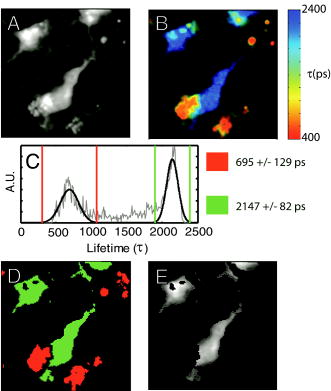 3.3.Separating a Fluorescence Energy Transfer Lifetime when it Overlaps with Autofluorescence in Human TissueIn some cases, particularly when a FRET interaction is taking place, the apparent lifetime of the background AF can be similar in distribution to one of the lifetimes of interest. Even in this case, it is often possible to separate the contributions of the lifetime due to FRET lifetime and the AF. As an initial proof of principle, postmortem human cortical sections from the temporal lobe of an Alzheimer patient [Fig. 3a ] were immunolabeled with A488, using the N-tau antibody. Cy3 was then added via a tertiary antibody, to ensure FRET. The lifetime of the A488 in the absence of Cy3 was obtained from cells stained with donor alone, using MUGLE, and found to be (Data not shown). A biexponential fit was performed using SPCImage with the longer lifetime fixed at this value. The distribution of [Fig. 3b], which contains the FRET quenched lifetime, was then analyzed using MUGLE [Fig. 3c]. As can be seen, two peaks in the lifetime distribution can be fit. The sample was then donor dequenched by photobleaching the acceptor fluorophore by repeatedly scanning the sample with 543-nm light at high intensity until Cy3 was no longer visible; A488 increased in intensity due to dequenching [Fig. 3d]. The brightness of the green/cyan-colored pixels clearly decreased [Fig. 3e] and MUGLE analysis shows that one of the peaks disappears [Fig. 3f] while the other survives, albeit with a slightly lower mean value and narrower Gaussian. This experiment was taken to confirm that the two peaks represent those pixels that are contaminated with autofluorescence and exogenous fluorophore exhibiting FRET, respectively. Photobleaching the acceptor removes the FRET component and does not affect the autofluorescence. The cause of the slight shortening of the autofluorescent peak is most likely because those pixels contain a mixture of both autofluorescence and fluorophore before bleaching. The red pixels in the segmentation shown in Fig. 3g closely match the spatial distribution of the remaining fluorescence in Fig. 3h, thereby validating our method further. Fig. 3(a) A neurofibrillary tangle in a neuron, immunolabeled with A488 (N-term) and Cy3. (b) The Lifetime image, prior to photobleaching, shows a suspected area of autofluorescence (white arrow). (c) MUGLE analysis shows two clear and distinct peaks at and . To validate that the shorter peak represents autofluorescence and the longer one FRET, the acceptor was photobleached to eliminate FRET. (d) The intensity of donor fluorophore increases after acceptor bleaching. (e) The region of autofluroesence appears to survive the irradiation, although the nonautofluorescent region is much dimmer. (f) MUGLE analysis of the postquench sample confirms that there is now only one peak. (g) The prebleach and (h) postbleach segmented images are also shown.  In a second and more challenging experiment, similar sections [Fig. 4a ] were immunolabeled with A488, using N-tau; and Cy3, using Alz50 (see Methods in Sec. 2). Alz50 is believed to be a conformation-specific antibody that recognizes tau only when it is folded, such that the microtubule binding domain (aa312-342) comes into close proximity with the N-terminal. We hypothesized that fluorophores attached to Alz50 and an N-terminal epitope (amino acids 2-13) would be close enough to support FRET if this interpretation of Alz50 conformational specificity is correct. If so, we predicted that A488 would interact with the Cy3, as they are both attached to the tau protein when tau is folded in such a way as it can aggregate to form a tangle. Fig. 4(a) A neurofibrillary tangle in a neuron, immunolabeled with A488 (N-term) and Cy3 (Alz50). (b) The shorter component of a biexponential fit contains Gaussians from the FRET lifetime and autofluorescence. Three moderate-sized autofluorescent aggregates (lipofuscin, an endogenous fluorophore) are indicated with arrows. The unquenched lifetime was fixed . (c) MUGLE analysis assumes two closely overlapping distributions. (d) The image is segmented based on the probability distributions, and the red distribution conforms well to the locations of the autofluorescence as verified through visual inspection. (e) The autofluorescence spatial distribution was used to make a mask and eliminate pixels from the original intensity image that corresponds to autofluorescence.  The lifetime distribution seems to result from two overlapping Gaussians [Fig. 4c], one of which can be characterized as , and the other as . A KS test of the data shows that it does not originate from a single normal distribution . By segmenting the tau tangle based on the most likely distribution that each pixel originates from [Fig. 4d], we see that the slightly shorter-lived Gaussian mainly originates from the AF on the left of the neuron and the two small inclusions shown with arrows, as confirmed by visual inspection of the cell using wide-field microscopy. The segmentation can then be used to mask the AF from the original image [Fig. 4e]. We propose that this method allows us to accurately extract the correct FRET lifetime from the experiment in spite of the fact that it is confounded by AF. 3.4.Use of Goodness-of-Fit-Based Filtering to Establish the Presence of Fluorescence Energy TransferThe presence of AF not only confounds the accurate measurement of lifetimes but also makes it difficult to show that a particular FRET interaction is taking place. AF masquerading as exogenous fluorphores with shortened lifetimes due to FRET sometimes make negative controls appear frustratingly similar to experimental samples, even when no acceptor is present. Figure 5 depicts filtering of the same dataset used in Fig. 4. The results of a monoexponential fit is shown in Fig. 4a, with the associated [Fig. 3b]. The scale is compressed to show the contrast between . The same three autofluorescent aggregates that were previously seen in Fig. 4 can be seen as regions of relatively high . Two pixels of interest are marked D and E in Fig. 5b. A cutoff of was selected empirically to give the best balance between elimination of AF and preservation of nonperturbed pixels and then consistently applied across all samples. The result of this filtration can be seen in Fig. 4c, which shows the shorter component of the biexponential fit after the mask was applied. For closer comparison, the time courses of nonautofluorescent and autofluorescent [Figs. 5d and 5e, labeled D and E in Fig. 5b], pixels are shown. We can see that even in the case of a sample that is expected to exhibit FRET, the monoexponential fit performed by SPCImage yields a reasonably low , compared to the autofluorscent pixel . It seems that the autofluorescent aggregate exhibits a highly nonexponential decay, which fits very poorly. In contrast, if we apply a biexponential model, very little contrast is observed ( for pixel D, for pixel E) (data not shown). Fig. 5An example of goodness-of-fit filtering. (a) The same sample used in Fig. 4 was fit pixel-wise with a monoexponential. (b) The associated map shows that the previously identified regions of AF have markedly higher than non-AF regions. A value of was chosen that best eliminated the AF pixels while preserving the non-AF pixels by comparison with visual inspection using wide-field microscopy. (c) This mask was then applied to the biexponential fitted data to retrieve more accurate values of and . The decay curves for (d) a non-AF and (e) AF pixel are shown to show how the strongly nonexponential decay of the AF pixels leads to high .  Multiple cells ( from three sections) were analyzed in this fashion, with the same number of negative controls consisting of cells labeled only with donor fluorophore, and positive controls in which the donor was immunolabeled with the acceptor via a tertiary antibody. The average as given by SPCImage (Fig. 6) fails to show significance between experimental condition and negative control . After filtering, statistical significance between experimental and negative control is achieved . It is clear that the improvement is mostly due to the reduction in the mean value and variability of for the negative control. Goodness-of-fit filtering allows statistical significance to be achieved for this low value of N (Fig. 6 ) Fig. 6Goodness-of-fit filtering allows apparent percentage of interacting molecules in the negative control data for tau conformationally FRET experiments inside aged human brain slices. The apparent percentage of interacting molecules as defined by the percentage contribution of the shorter lifetime component is shown for the following conditions. The leftmost bar shows for the experimental condition, in which A488 (N-term) is expected to FRET when tau is aggregated with Cy3 (epitope 50). The second bar is a control, where the A488-N-term antibody is directly immunolabelled with Cy3. The two bars on the right are the control prior to goodness-of-fit filtering and after filtering. Stars are shown above bars that are significantly different in the experimental condition. ( for unfiltered, for filtered). Goodness-of-fit filtering allows statistical significance to be achieved for this dataset in a setting where noise from autofluorescence would otherwise preclude detecting FRET.  4.DiscussionThe data here show that tau protein in intracellular tangles in AD can be immunolabeled using N-tau and the conformationally dependent antibody, Alz50. Alz50 recognizes a discontinuous epitope on the tau molecule and therefore has been suggested to bind only when the protein is in a specific conformation, which happens during tangle formation.28 It is therefore possible to categorically show the presence or absence of a particular conformation using FLIM microscopy in aged human brain tissue. Further, the use of FLIM to detect intermolecular distance is well established.29 With the accurate measurement of changes in lifetime due to FRET, studies of differences in protein conformation or protein interactions become easier and more reliable. The two techniques presented here both concern the masking of AF in FRET/FLIM studies using exogenous fluorophores or FPs; however, they have two slightly different applications. The MUGLE technique is solely concerned with accurately measuring the lifetime of a sample in the presence of AF and could also be used to separate multiple, spatially segregated lifetimes within a sample, for example, if FRET efficiency was greater in one cellular compartment than in another. The probabilistic segmentation of the image allows us to produce a quantized image of the spatial distributions of populations of fluorophores based on their lifetimes, again provided that those lifetimes are well represented by discrete peaks. MUGLE does not enhance the resolution of FLIM microscopy per-se, but allows spatially segregated components to be separated even if the distributions overlap. Presently, data of this type are often analyzed by attempting to manually select limits on either side of peaks in the lifetime distribution. This technique is highly subjective and biased if the peaks overlap, leading to poor estimates of FRET efficiency. MUGLE offers the advantage of being objectively based on a numerical technique that minimizes to a single result and is therefore less prone to user influence. As our numerical simulations show, however, there is still a larger level of uncertainty in cases where the Gaussians overlap due to larger errors, although the mean values over several experimental samples are expected to be accurate. These observations taken together suggest that if, for example, we extended the pilot study of tau conformation to compare animals at different ages, and tried to compare FRET efficiencies, we might find that higher values of n were required if the Gaussians overlap than if they did not. The companion technique, goodness-of-fit filtering, provides a mechanism for improving the effective signal to noise in a FLIM measurement by disregarding the pixels that are contaminated with AF. By directly identifying the pixels that contain AF, there is no requirement that the lifetimes fall into separable distribution and no need to establish the identity of the distributions using donor dequenching. In summary, goodness-of-fit filtering allows us to establish the existence of FRET, while MUGLE extracts lifetime distributions. The two techniques could be used in tandem by initially demonstrating the existence of FRET interaction using goodness-of-fit filtering, with MUGLE used to better quantify the FRET efficiency. Alternatively, the two independent techniques can be used to separately measure the spatial location of AF aggregates, thereby adding confidence that MUGLE was being used to correctly segregate lifetimes in cases where the distribution cannot be shown to be non-normal using a KS test. It is worth noting that in our use of MUGLE, the dataset was shown to be non-normal using the KS test, thereby validating the fitting of more than one Gaussian without the aid of goodness-of-fit filtering. MUGLE can also be used to extract multiple average lifetimes from spatially segregated populations of fluorophores with different lifetimes due to protein interaction or conformation differences. In this case, goodness-of-fit filtering could be used to mask out likely AF signals and make the distributions easier to fit. The results can be used to segment the image and compare the locations of populations with the locations of cellular compartments. As of yet, attempts at generating reliable lifetime data in whole animal brain have been challenging, owing to AF. These techniques could potentially be applied to in-vivo FLIM. It may be possible to observe protein interactions in the intact functioning brain and assess the conformational differences between isoforms of proteins that are important to neurodegenerative and other diseases. Since both techniques are postprocessing segmentation tools, when used to account for AF as a confound, they necessarily involve discarding the pixels that contain AF to improve the overall quality of the data. To avoid discarding information, account of AF would have to be taken at the analysis or preprocessing stage. Since the simple exponential function is a poor representation of the decay profile of autofluorescence,16 performing a triexponential fit does not account for AF well. In addition, multiexponential fitting is an ill-posed problem, meaning that it becomes increasingly difficult to arrive at a single answer with any confidence as the number of fitting parameters increases. A solution to this problem would involve a data preprocessing step that does not rely on curve fitting. 5.ConclusionMUGLE offers a method of postprocessing for FLIM data that allows more quantitative measurements of lifetimes, especially in the presence of confounds like AF. MUGLE may also be useful in situations where spatially segregated fluorophores of different lifetimes exist or when proteins interact with varying closeness in different cellular compartments. A limitation of the approach is that while it is possible to separate fluorophores by their lifetime means and widths, the identification of the fluorophore can only be done by comparing the segmented image with the original or by imaging the cell using different combinations of excitation and emission filters, in an attempt to identify the populations. With that in mind, we also propose that AF can be filtered out due to its comparatively poor fit to the monoexponential decay model. We show that through elimination of AF, we achieve statistical significance between negative controls and experimental samples where it could not be achieved without filtering. These two techniques may be used separately or together to help elucidate FLIM data that are otherwise difficult to interpret. AcknowledgmentsThe authors acknowledge financial support from the National Institutes of Health (NNS10828, AG08487, AG12406, AI068871, AG026240, AG026593, EB00768, AG026249, and AG08487-16) and the Dana Foundation. ReferencesP. R. Selvin,
“The renaissance of fluorescence resonance energy transfer,”
Nat. Struct. Biol., 7
(9), 730
–734
(2000). https://doi.org/10.1038/78948 1072-8368 Google Scholar
R. Y. Tsien,
“Breeding and building molecules to spy on cells and tumors,”
Keio J. Med., 55
(4), 127
–140
(2006). 0022-9717 Google Scholar
K. Konig,
P. T. So,
W. W. Mantulin,
B. J. Tromberg, and
E. Gratton,
“Two-photon excited lifetime imaging of autofluorescence in cells during UVA and NIR photostress,”
J. Microsc., 183
(pt 3), 197
–204
(1996). 0022-2720 Google Scholar
G. J. Brakenhoff,
J. Squier,
T. Norris,
A. C. Bliton,
M. H. Wade, and
B. Athey,
“Real-time two-photon confocal microscopy using a femtosecond, amplified Ti:sapphire system,”
J. Microsc., 181
(pt 3), 253
–259
(1996). https://doi.org/10.1046/j.1365-2818.1996.97379.x 0022-2720 Google Scholar
J. R. Lakowicz,
I. Gryczynski,
H. Malak,
M. Schrader,
P. Engelhardt,
H. Kano, and
S. W. Hell,
“Time-resolved fluorescence spectroscopy and imaging of DNA labeled with DAPI and Hoechst 33342 using three-photon excitation,”
Biophys. J., 72
(2 pt 1), 567
–578
(1997). 0006-3495 Google Scholar
B. J. Bacskai,
J. Skoch,
G. A. Hickey,
R. Allen, and
B. T. Hyman,
“Fluorescence resonance energy transfer determinations using multiphoton fluorescence lifetime imaging microscopy to characterize amyloid-beta plaques,”
J. Biomed. Opt., 8
(3), 368
–375
(2003). https://doi.org/10.1117/1.1584442 1083-3668 Google Scholar
M. J. Cole,
J. Siegel,
S. E. Webb,
R. Jones,
K. Dowling,
M. J. Dayel,
D. Parsons-Karavassilis,
P. M. French,
M. J. Lever,
L. O. Sucharov,
M. A. Neil,
R. Juskaitis, and
T. Wilson,
“Time-domain whole-field fluorescence lifetime imaging with optical sectioning,”
J. Microsc., 203
(pt 3), 246
–257
(2001). https://doi.org/10.1046/j.1365-2818.2001.00894.x 0022-2720 Google Scholar
W. Becker,
A. Bergmann,
E. Haustein,
Z. Petrasek,
P. Schwille,
C. Biskup,
L. Kelbauskas,
K. Benndorf,
N. Klocker,
T. Anhut,
I. Riemann, and
K. Konig,
“Fluorescence lifetime images and correlation spectra obtained by multidimensional time-correlated single photon counting,”
Microsc. Res. Tech., 69
(3), 186
–195
(2006). https://doi.org/10.1002/jemt.20251 1059-910X Google Scholar
M. Peter,
S. M. Ameer-Beg,
M. K. Y. Hughes,
M. D. Keppler,
S. Prag,
M. Marsh,
B. Vojnovic, and
T. Ng,
“Multiphoton-FLIM quantification of the EGFP-mRFP1 FRET pair for localization of membrane receptor-kinase interactions,”
Biophys. J., 88
(2), 1224
–1237
(2005). https://doi.org/10.1529/biophysj.104.050153 0006-3495 Google Scholar
O. Berezovska,
P. Ramdya,
J. Skoch,
M. S. Wolfe,
B. J. Bacskai, and
B. T. Hyman,
“Amyloid precursor protein associates with a nicastrin-dependent docking site on the presenilin 1-gamma-secretase complex in cells demonstrated by fluorescence lifetime imaging,”
J. Neurosci., 23
(11), 4560
–4566
(2003). 0270-6474 Google Scholar
O. Berezovska,
A. Lleo,
L. D. Herl,
M. P. Frosch,
E. A. Stern,
B. J. Bacskai, and
B. T. Hyman,
“Familial Alzheimer’s disease presenilin 1 mutations cause alterations in the conformation of presenilin and interactions with amyloid precursor protein,”
J. Neurosci., 25
(11), 3009
–3017
(2005). https://doi.org/10.1523/JNEUROSCI.0364-05.2005 0270-6474 Google Scholar
V. Calleja,
S. M. Ameer-Beg,
B. Vojnovic,
R. Woscholski,
J. Downward, and
B. Larijani,
“Monitoring conformational changes of proteins in cells by fluorescence lifetime imaging microscopy,”
Biochem. J., 372
(pt 1), 33
–40
(2003). 0264-6021 Google Scholar
P. B. Jones,
L. Herl,
O. Berezovska,
A. T. N. Kumar,
B. J. Bacskai, and
B. T. Hyman,
“Time-domain fluorescent plate reader for cell based protein-protein interaction and protein conformation assays,”
J. Biomed. Opt., 11
(5), 054024
(2006). https://doi.org/10.1117/1.2363367 1083-3668 Google Scholar
M. Peter and
S. M. Ameer-Beg,
“Imaging molecular interactions by multiphoton FLIM,”
Biol. Cell, 96
(3), 231
–236
(2004). 0399-0311 Google Scholar
M. Tramier,
M. Zahid,
J. C. Mevel,
M. J. Masse, and
M. Coppey-Moisan,
“Sensitivity of CFP/YFP and GFP/mCherry pairs to donor photobleaching on FRET determination by fluorescence lifetime imaging microscopy in living cells,”
Microsc. Res. Tech., 69
(11), 933
–939
(2006). https://doi.org/10.1002/jemt.20370 1059-910X Google Scholar
D. Elson,
J. Requejo-Isidro,
I. Munro,
F. Reavell,
J. Siegel,
K. Suhling,
P. Tadrous,
R. Benninger,
P. Lanigan,
J. McGinty,
C. Talbot,
B. Treanor,
S. Webb,
A. Sandison,
A. Wallace,
D. Davis,
J. Lever,
M. Neil,
D. Phillips,
G. Stamp, and
P. French,
“Time-domain fluorescence lifetime imaging applied to biological tissue,”
Photochem. Photobiol. Sci., 3
(8), 795
–801
(2004). https://doi.org/10.1039/b316456j 1474-905X Google Scholar
J. A. Jo,
Q. Fang,
T. Papaioannou,
J. D. Baker,
A. H. Dorafshar,
T. Reil,
J. H. Qiao,
M. C. Fishbein,
J. A. Freischlag, and
L. Marcu,
“Laguerre-based method for analysis of time-resolved fluorescence data: application to in-vivo characterization and diagnosis of atherosclerotic lesions,”
J. Biomed. Opt., 11
(2), 021004
(2006). https://doi.org/10.1117/1.2186045 1083-3668 Google Scholar
D. B. McCombie,
A. T. Reisner, and
H. H. Asada,
“Laguerre-model blind system identification: cardiovascular dynamics estimated from multiple peripheral circulatory signals,”
IEEE Trans. Biomed. Eng., 52
(11), 1889
–1901
(2005). 0018-9294 Google Scholar
W. Press,
B. Flannery,
S. Teukolsky, and
W. Vetterling, Numerical Recipes in C: The Art of Scientific Computing,
(1992) Google Scholar
H. Yokoe and
T. Meyer,
“Spatial dynamics of GFP-tagged proteins investigated by local fluorescence enhancement,”
Nat. Biotechnol., 14
(10), 1252
–1256
(1996). 1087-0156 Google Scholar
M. Tsuchida,
T. Miura, and
K. Aibara,
“Lipofuscin and lipofuscin-like substances,”
Chem. Phys. Lipids, 44
(2-4), 297
–325
(1987). 0009-3084 Google Scholar
J. L. Jankowsky,
H. H. Slunt,
V. Gonzales,
N. A. Jenkins,
N. G. Copeland, and
D. R. Borchelt,
“APP processing and amyloid deposition in mice haplo-insufficient for presenilin 1,”
Neurobiol. Aging, 25
(7), 885
–892
(2004). 0197-4580 Google Scholar
H. F. Trotter,
“An elementary proof of the central limit theorem,”
Arch. Math., 10
(226–234),
(1959). 0003-889X Google Scholar
V. A. Lorenz-Fonfria and
H. Kandori,
“Transformation of time-resolved spectra to lifetime-resolved spectra by maximum entropy inversion of the laplace transform,”
Appl. Spectrosc., 60
(4), 407
–417
(2006). 0003-7028 Google Scholar
G. Wang,
Y. Gao, and
M. L. Geng,
“Analysis of heterogeneous fluorescence decays in proteins. Using fluorescence lifetime of 8-anilino-1-naphthalenesulfonate to probe apomyoglobin unfolding at equilibrium,”
Biochim. Biophys. Acta, 1760
(7), 1125
–1137
(2006). 0006-3002 Google Scholar
J. A. Nelder and
R. Mead,
“A simplex method for function minimization,”
Comput. J., 7 308
–313
(1965). 0010-4620 Google Scholar
K. C. B. Lee,
J. Siegel,
S. E. D. Webb,
S. Lévéque-Fort,
M. J. Cole,
R. Jones,
K. Dowling,
M. J. Lever, and
P. M. W. French,
“Application of the stretched exponential function to fluorescence lifetime imaging,”
Biophys. J., 81
(3), 1265
–1274
(2001). 0006-3495 Google Scholar
F. Garcia-Sierra,
N. Ghoshal,
B. Quinn,
R. W. Berry, and
L. I. Binder,
“Conformational changes and truncation of tau protein during tangle evolution in Alzheimer’s disease,”
J. Alzheimers Dis., 5
(2), 65
–77
(2003). Google Scholar
H. Wallrabe and
A. Periasamy,
“Imaging protein molecules using FRET and FLIM microscopy,”
Curr. Opin. Biotechnol., 16
(1), 19
–27
(2005). https://doi.org/10.1016/j.copbio.2004.12.002 0958-1669 Google Scholar
|


