

|
|
1.IntroductionGlaucoma is an optic neuropathy that causes the loss of retinal ganglion cells and damage to the retinal nerve fiber layer (RNFL). It causes progressive and irreversible vision loss if left untreated. The early detection of glaucoma is important because glaucoma progresses even before visual field loss occurs.1 Visual field test and ophthalmoscopic assessment of an optic nerve head are subjective methods to diagnose glaucoma. Since the thinning of RNFL is a direct indicator of glaucoma, glaucoma can also be diagnosed by objective measurement of RNFL thickness. Objective and quantitative measurements of RNFL have certain advantage over the subjective methods because in these methods, the intervention of experts becomes unnecessary and statistical diagnostic analysis is possible. Therefore, methods such as optical coherence tomography (OCT) and scanning laser polarimetry (SLP) have been utilized. OCT is a low-coherence interferometry technique that can provides images of biological tissues with a resolution of the order of a few micrometers.2 Schuman first measured the thickness of RNFL by OCT.3 Thickness measurement using OCT images has certain limitations, namely, the requirement of high axial resolution and a high-quality algorithm for boundary segmentation. GDx-VCC (Carl Zeiss Meditec) is a commercially available SLP that provides an RNFL thickness map by converting the phase retardation of RNFL, assuming that the birefringence of RNFL is constant.4, 5 It compensates for the corneal birefringence by monitoring a bow-tie pattern in the macular region and measures the combined effect of the thickness and birefringence of RNFL and diagnoses glaucoma statistically using the normative database.6 Polarization-sensitive optical coherence tomography (PS-OCT) has been developed to measure the depth-resolved birefringence of biological samples.7, 8 By using PS-OCT, an in vivo human retina was first examined by Cense 9 Pircher showed polarization scrambling at the retinal pigment epithelium in the macular region.10 The recent development of spectral-domain OCT (SD-OCT) revealed that SD-OCT had a higher signal-to-noise ratio than the conventional time-domain OCT.11, 12 By using high-speed and highly sensitive SD-OCT, it is possible to measure a three-dimensional (3-D) retina in vivo.13 The first demonstration of polarization-sensitive spectral-domain OCT (PS-SD-OCT) was reported by Yasuno 14 High-speed retinal SD-OCT was adapted to PS-OCT by Cense 15 Götzinger demonstrated 3-D phase retardation images and optic axis images of the retina by using the free-space PS-SD-OCT system.16 One characteristic of PS-OCT is that corneal birefringence compensation is possible by using the surface signal.17, 18, 19 In retinal imaging, the signal from the anterior boundary of the retina can be used as the surface signal. Unlike SLP, this corneal compensation does not rely on healthy macula. The other characteristic is the ability to measure the thickness and birefringence of RNFL simultaneously. Cense showed that the birefringence of RNFL has angular dependence around the optic nerve head.20, 21 Mujat showed an en face birefringence map of RNFL for the first time.22 In contrast, SLP measures the en face phase retardation map, that is, the combined effect of the thickness and birefringence of RNFL. Although by using PS-OCT it is possible to measure thickness and birefringence separately, birefringence measurement is less reliable in the case of a thin RNFL.15, 20 In addition, the diagnostic performance of PS-OCT with regard to glaucoma has not yet been demonstrated. Since it is known that SLP gives a good performance in the diagnosis of glaucoma,23, 24, 25 a comparison of PS-OCT and SLP is of significant interest in the preliminary research on the detection of glaucoma using PS-OCT. Previously, Huang measured birefringence of RNFL by using thickness measured by conventional OCT and phase retardation measured by SLP.26 Wojtkowski compared a thickness map of RNFL measured by SD-OCT and a phase retardation map measured by SLP.27 However, there is still no report about the comparison of PS-OCT and SLP. In this paper, we describe a pilot study on the quantitative comparison of the phase retardation of RNFL using PS-OCT and SLP for both healthy and glaucomatous eyes. 2.Methods2.1.PS-SD-OCT SystemThe details of the PS-SD-OCT system employed in this study have been described in Ref. 28. In brief, the schematic diagram of our system is shown in Fig. 1 . Fig. 1Diagram of the PS-SD-OCT system. The following notations are used: SLD—superluminescent diode; PC—polarization controller; ND—neutral density filter; LP—linear polarizer; EO—electro-optic modulator; M—mirror; G—grating; PBS—polarizing beamsplitter; CCD—line-CCD camera.  The light source is a superluminescent diode with a central wavelength of , a bandwidth of , and an experimental axial resolution of in air. After the polarization is vertically aligned by a linear polarizer (LP), an electro-optic (EO) modulator with a fast axis of modulates the incident polarization state. The incident beam is coupled into a fiber coupler, the splitting ratio of which is . The LP in the reference arm provides constant amplitude and constant relative phase between the two orthogonal polarizations at the spectrometer, independent of the incident state of the polarization. In the sample arm, the beam is scanned by the two-axis galvanoscanner mirror. An imaging plane made by the objective lens is relayed by a Volk ophthalmic lens (78D) to the retina. The probing power is . The backscattered signal from the retina is coupled into the fiber again and detected by the polarization-sensitive spectrometer. The spectrometer contains a polarizing beamsplitter and two line-CCD cameras in order to detect the horizontal and vertical polarization channels simultaneously. The line trigger for both cameras is synchronized with the EO modulator. The incident polarization is modulated as a three-step function in order to embed the polarimetric property into the B-scan. Two power spectra detected by the two CCD cameras are individually inverse-Fourier transformed to obtain two phase-resolved OCT signals. By using the spatial frequency components of the OCT signals, all the elements of the Jones matrix of the sample arm are obtained. The matrix diagonalization method developed by Park is used in order to compensate for the birefringence of the single-mode fiber and the cornea.19 Last, the phase retardation, relative orientation, and diattenuation of the sample are calculated. 2.2.Three-Dimensional Volumetric Measurement by PS-SD-OCTSince the RNFL in the peripheral region contains nerve fibers that are all diverging from the optic nerve head, SLP diagnoses glaucoma by measuring the en face phase retardation of RNFL in the peripheral region. By using our PS-SD-OCT system, the (3-D) intensity and phase retardation volumes in the peripheral region are measured. The measurement range is on the retina. The probe beam is scanned from the nasal to the temporal regions with 1023 A-lines for each B-scan. The lateral density of the A-lines is , which is well below the lateral spot size of our system, that is, . This setup is attributed to the high dense scan required for PS-OCT with multiple incident polarizations.29 The raster scanning from inferior to superior is performed with 140 B-scans in . This protocol is used for all PS-SD-OCT measurements described in this paper. 2.3.En Face Phase Retardation MapsTo compare the en face phase retardation maps of SLP and PS-SD-OCT, the 3-D phase retardation volume measured by PS-SD-OCT was shrunk into the en face map using the following comparable method. The main contribution to the SLP signal is high scattering from the layers beneath the RNFL, such as the interface of the inner and outer segments of the photoreceptor layers (IPRL) and the retinal pigment epithelium (RPE). Thus, it is reasonable to extract the backscattered signal from these high-scattering layers in the PS-SD-OCT images in order to compare these two systems. The cumulative phase retardation of PS-OCT from the lower layers corresponds to the double-pass phase retardation of the RNFL because there is no birefringent tissue between the posterior boundary of RNFL and RPE.16, 30 It is known that RPE has polarization scrambling in the macula.10, 16 The detail of polarization scrambling in the peripheral region has not been studied yet. In our experiment, polarization scrambling was not observed at the RPE on the periphery of the optic nerve head, as shown in Fig. 2c . Since RPE has the strongest signal in the retinal image, the segmentation of the RPE layer is stable and easy. Hence, in this paper, we extract the signal from the RPE in the PS-SD-OCT images to make an en face phase retardation map. However, some studies have reported polarization scrambling in the peripheral region,16, 31 and it is not always guaranteed that our method is applicable. Other highly backscattering layers, e.g., IPRL, would be candidates to avoid possible polarization scrambling for the future version of this method. Fig. 2Intensity image (a), double-pass cumulative phase retardation image (b), and composite image (c) of inferior of an optic nerve head of a healthy human left eye. The image size is . The longitudinal scale is enlarged to twice the lateral scale. The range of the phase retardation is from 0 to radians (0 to ) in a double pass. The white arrows in (b) and (c) indicate an artificial phase retardation in the blood vessel. A red line over the intensity image in (d) indicates the segmented RPE layer. (Color online only.)  The large white and yellow spots in Figs. 2b and 2c (indicated by arrows) are phase retardation artifacts caused by Doppler signal of the blood flow. In our algorithm of PS-SD-OCT, we cannot discriminate the phase change caused by Doppler flow from real birefringence. However, this artifact is localized in a blood vessel and does not affect the phase retardation of the RPE. In order to extract the phase retardation at the RPE, first the RPE layer is segmented from the intensity images. For this purpose, the maximum gradient points are detected below the anterior boundary of the retina and smoothed to interpolate the shadow of blood vessels for each B-scan intensity image.32 Figure 2d shows the segmented RPE; it indicates that our segmentation algorithm works well. Even if the detected layer is slightly deviated—for example, an IPRL was falsely selected—the phase retardation does not change drastically [Fig. 2b]. This is because the alternation of the phase retardation occurs in the RNFL, and the small fluctuation of the segmentation does not affect to the detected phase retardation value. No smoothing algorithm was employed for the phase retardation images. The same procedure is applied to all B-scan stacks, and an en face phase retardation map at the RPE position is obtained. 2.4.Quantitative Analysis of Phase RetardationFor the quantitative comparison of PS-SD-OCT and SLP, the cumulative phase retardation of the RNFL in the peripheral region is examined because nerve fibers diverge from the optic nerve head. For this purpose, the phase retardation around the optic nerve head is extracted from the en face phase retardation map. GDx-VCC has a function that shows the RNFL thickness curve in the annular area of the en face phase retardation map. The RNFL thickness curve measured by GDx-VCC was converted to the double-pass phase retardation33 by using a conversion factor of . An annular area with an outer radius of and an inner radius of was set in order to extract the phase retardation of PS-SD-OCT; this setting is identical to that used in GDx-VCC. We evaluated two methods for calculating the phase retardation curve of PS-SD-OCT. In the first simple method, the phase retardation of PS-SD-OCT in the annular area was calculated using a simple moving average with a kernel size of . Second, the following histogram-based method is also evaluated as an alternative to the first method. Histograms of small angular areas within the ring are obtained, and the mode value of the histogram is calculated. The small angular area is moved along the circumference, and the mode values are calculated for each small angular area. After a moving average with a kernel of , the phase retardation curve is obtained. 3.Results and Discussion3.1.SubjectsAll experiments were performed using a protocol that adheres to the tenets of the Declaration of Helsinki and that was approved by the Institutional Review Board of the University of Tsukuba and Tokyo Medical University. As the healthy subject, a volunteer (25-year-old Japanese male) without any detectable ocular disease was selected. As the glaucoma subject, a volunteer (42-year-old Japanese male) with glaucoma was selected. For both volunteers, the left eyes were examined. 3.2.Three-Dimensional Phase Retardation VolumeFigure 3 shows the 3-D intensity and phase retardation image measured by PS-SD-OCT in the retinal peripheral region of the retina. The figure on the left in Fig. 3 shows the phase retardation volume with a front view from the anterior side, while the one on the right shows the rear view from the posterior side. The hue of its color bar corresponds to the phase retardation from 0 to , while the opacity corresponds to the intensity. Fig. 3Front view (left) and rear view (right) of the three-dimensional (3-D) phase retardation image of a healthy eye in the peripheral region. A measurement range of was scanned on the sample. The hue of the color bar is same as that in Fig. 2. (Color online only.) 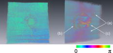 Several structures were observed in the 3-D phase retardation map similar to the previous report.16 In the front view of Fig. 3, the phase retardation was nearly zero because fiber-optic and corneal birefringence, which causes phase retardation artifacts in the retina, was compensated using a reference signal of the retinal surface.34, 35 In the inferior and superior regions, the high phase retardation beneath the surface was visible because the volume image was semitransparent. In the rear view, the double-hump pattern of the phase retardation was observed in the superior and inferior regions of the optic nerve head (a). The phase retardation also changed at the temporal edge of the optic nerve head (scleral canal rim; b) and the lamina cribrosa in the optic nerve head (c). Figure 4 shows the en face phase retardation maps on the surface of retina. For better visualization, a high threshold was set in order to segment the first intensity peak on the surface rather than the boundary between the noise and signal areas. The phase retardation map of the glaucomatous eye had higher speckle noise than that of the healthy eye. In both maps, the phase retardation had high values at the edge of the optic disk because of an error of the surface segmentation. Since there was no radial variation of the phase retardation, the residual effect of the fiber-optic and corneal birefringence could be negligible. Figure 5 shows the histogram of the phase retardation on the surface of retina. The mode values of the healthy and glaucomatous eyes were and , respectively. Since all noise near zero retardation affects the result to a positive direction, the histogram had asymmetric distribution and the phase retardation diverged from zero. Fig. 4Phase retardation maps of the healthy eye (left) and glaucomatous eye (right) on the surface of the retina. 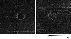 Fig. 5Histograms of the phase retardation of the healthy eye (solid line) and glaucomatous eye (dashed line) on the surface of the retina.  Figure 2 shows the intensity (a) and phase retardation (b) images of a healthy human retina at the superior uppermost B-scan in Fig. 3. The retinal layers are clearly visible in the intensity image, similar to the previous report.20 In the thick RNFL area, the phase retardation evidently changes. It has a noisy appearance in a low-intensity area such as the outer nuclear layer and shadow beneath the retinal blood vessels. Figure 2c is the composite image of the intensity and phase retardation images. In the composite image, the hue corresponds to the phase retardation, while the brightness corresponds to the intensity. In the composite image, the phase retardation with high signal intensity is shown in a bright color. Hence, both intensity and phase retardation can be viewed in one image. This color map is also used for the en face phase retardation map in the following sections. 3.3.Healthy EyeFigure 6 shows the en face phase retardation maps of GDx-VCC (b) and PS-SD-OCT (d) of a healthy human volunteer. The annular areas for the quantitative analysis are indicated by gray and white circles in Figs. 6b and 6d, respectively. The fundus image (a) and OCT projection image (c) are also shown. The OCT projection image was calculated by summing each A-line of the linear OCT intensity signal. The en face phase retardation images of both GDx-VCC and PS-SD-OCT showed a similar double-hump pattern, which is consistent with the typical distribution of RNFL of healthy eyes. Fig. 6Fundus image (a), nerve fiber thickness map measured by GDx-VCC (b), en face projection image of the OCT intensity (c), and en face phase retardation image measured by the PS-SD-OCT (d) for the healthy eye. The fundus image was measured by a nonmydriatic fundus camera. Measurement ranges of and were scanned on the sample for GDx-VCC and PS-SD-OCT, respectively. An annular area indicated by two white circles in the phase retardation image of PS-SD-OCT is used to calculate the graph of the phase retardation shown in Fig. 7. 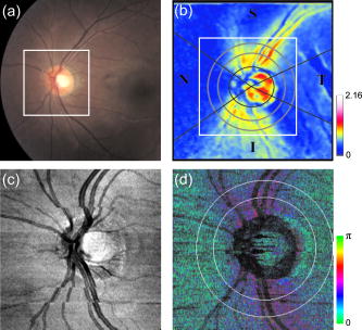 Fig. 7The upper image shows the OCT intensity at the center of the peripheral annular area of the healthy eye. The middle image shows the phase retardation image at the same position of the upper intensity image. The axial range of these images is . The lower figure shows the round-trip cumulative phase retardation around the optic nerve head measured by PS-SD-OCT with simple averaging (dotted line), the histogram-based method (solid line), and GDx-VCC (dashed line). The notations used on the horizontal axis are as follows: T—temporal; S—superior; N—nasal; I—inferior.  Figure 7 shows the phase retardation curves of a healthy eye. The dotted line in Fig. 7 shows the phase retardation of PS-SD-OCT in the annular area calculated by the simple moving average. The curve takes extremely high values as compared to the curve of GDx-VCC. This is because the phase retardation ranges from 0 to and has a strongly asymmetric distribution. Therefore, averaging is not appropriate for this case. The phase retardation curve calculated by the second histogram-based method is shown in Fig. 7 by a solid line. The high phase retardation in the temporal and nasal regions obtained in the first method was decreased in the second method, which is reasonable because of the non-Gaussian distribution of the phase retardation. The curves of both PS-SD-OCT and GDx-VCC showed humps in the superior and inferior regions. In the case of PS-SD-OCT, the phase retardation inferior to the optic nerve head had the maximum value. Both the superior and inferior peaks of PS-SD-OCT were higher than that of GDx-VCC. Although the reason is not clear, the curve of GDx-VCC had a flatter shape in the inferior region. The uneven curve of PS-SD-OCT is a reasonable result of thick RNFL in the inferior region, as shown in the intensity image. To observe the correlation between the phase retardation and the retinal structure, the OCT intensity image at the center of the peripheral annular area is shown in the upper image of Fig. 7. The shadows beneath the retinal blood vessels are represented in the phase retardation graph as gray masks. The phase retardation had local peaks on one side or both sides of some blood vessels, as indicated by arrows in Fig. 7. The possible reason for this is that the phase retardation was affected by thick RNFL around the retinal blood vessels. In contrast, GDx-VCC did not show such sharp peaks in Fig. 7. However, we can see the peaks of the phase retardation in the en face phase retardation map measured by GDx-VCC in Fig. 6b. For example, there are three peaks in the temporal superior area of the calculation ring of Fig. 6b, but they are combined into a single peak in the curve of Fig. 7. This means that GDx-VCC also measures such peaks near blood vessels as PS-SD-OCT, but they are largely smoothed in the curve of Fig. 7. Therefore, the difference near blood vessels in Fig. 7 was caused by the difference between the calculation procedures of PS-SD-OCT and GDx-VCC. In order to check the birefringence of RNFL, we manually segmented the thickness of RNFL using the intensity image of Fig. 7 and calculated the double-pass phase retardation per unit depth (DPPR/UD). Figure 8 shows the thickness and DPPR/UD of the healthy eye. The DPPR/UD in the superior and inferior regions are higher than in the temporal and nasal regions. Both the thickness and the DPPR/UD are in the same order of that reported previously.20, 21 3.4.Glaucomatous EyeA glaucoma patient was also examined using the same scheme. Figure 9 shows the visual field test of the glaucomatous eye with the full threshold method on the central of the visual field. The glaucomatous eye has severe loss of inferior visual field and moderate loss of superior visual field. Fig. 9Visual field test of the glaucomatous eye measured using the Humphrey field analyzer II (Carl Zeiss Meditec) with full threshold method on the central of the visual field. 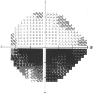 Figure 10 shows the en face phase retardation map of the glaucomatous eye measured by PS-SD-OCT and GDx-VCC. The lateral quick motion in the inferior region was manually compensated. The double-hump patterns of the glaucomatous eye obtained from both PS-SD-OCT and GDx-VCC were degraded as compared to that of the healthy eye shown in Figs. 6b and 6d. In the inferior region, GDx-VCC had a relatively higher phase retardation at the nasal side near the optic nerve head than PS-SD-OCT. Although the superior and inferior visual fields in Fig. 9 showed apparent differences, it is difficult to detect such differences in Figs. 10b and 10d. A quantitative comparison provides useful results. Fig. 10Fundus image (a), nerve fiber thickness map measured by GDx-VCC (b), en face projection image of the OCT intensity (c), and en face phase retardation image measured by PS-SD-OCT (d) for the glaucomatous eye. The fundus image was measured by a mydriatic fundus camera. The measurement range is the same as that shown in Fig. 6. Since the lateral quick motion in the inferior region of PS-SD-OCT images was manually compensated after the measurement, there are some empty spaces in (c) and (d).  Figure 11 shows the phase retardation curves and circular intensity image of the glaucomatous eye. The agreement between the phase retardation curves of PS-SD-OCT and GDx-VCC were significantly improved by the histogram-based method, while the curve calculated by a simple rolling average was not sufficient. In both the PS-SD-OCT and GDx-VCC curves, the superior phase retardation had a lower value than that of the inferior region. Again, the phase retardation measured by PS-SD-OCT had local peaks on one side of the retinal vessels, as indicated by arrows in Fig. 11. The values of the phase retardation curve of GDx-VCC were close to those of the PS-SD-OCT curve, excluding the sharp peaks near the blood vessels. As we described in the preceding subsection, this difference may be due to the different smoothing methods of PS-SD-OCT and GDx-VCC. Fig. 11The upper image shows the OCT intensity at the center of the peripheral annular area of the glaucomatous eye. The middle image shows the phase retardation image at the same position of the upper intensity image. The axial range of these images is . The lower figure shows the round-trip cumulative phase retardation around the optic nerve head measured by PS-SD-OCT with simple averaging (dotted line), the histogram-based method (solid line), and GDx-VCC (dashed line).  In PS-SD-OCT, the conventional 3-D OCT intensity volume is also acquired simultaneously with the phase retardation volume, which enables a direct structural observation of RNFL. Figure 12 shows the superior and inferior B-scan intensity images that are tangential to the inner circle of radius . The thinning of RNFL in the superior region was apparent, which is in agreement with the phase retardation measurements of PS-SD-OCT and GDx-VCC. The visual field test in Fig. 9 also supports the above-mentioned results, namely, the decreased phase retardation and thinning of RNFL measured by PS-SD-OCT and GDx-VCC. The thickness was manually segmented from the intensity image in Fig. 11, and the DPPR/UD was calculated for the glaucomatous eye, as shown in Fig. 13 . The posterior boundary of the RNFL was not clear compared to the healthy eye. Hence, Fig. 13 has poor reliability. The DPPR/UD was deviated, but this is a result of the unreliable thickness. The thickness measurement has to be improved using ultrahigh resolution and a sophisticated algorithm of the segmentation for the further investigation of the birefringence of glaucomatous eyes in the future. 3.5.Observation of the Phase Retardation by Polar PlotTo observe the distribution of the cumulative phase retardation intuitively, the polar plot of the phase retardation curve overlaid on the en face phase retardation map is shown in Fig. 14 . The center and outermost scale of the polar plot shows and , respectively. This polar plot shows the en face distribution of the phase retardation and the representative curve of the phase retardation in the annular area. The area of high phase retardation in the healthy eye broadens in both the superior and inferior regions. This representation is useful when normal and glaucomatous eyes are compared. Fig. 14Polar plot of the TSNIT phase retardation curve over the en face phase retardation map of the healthy eye. The origin of the polar plot was set at the center of the annular ring used to calculate the TSNIT curve. The range of the radial axis (phase retardation) is 0 to , with a scale.  Figure 15 shows the polar plot of the phase retardation of the glaucomatous eye. In contrast to the healthy eye shown in Fig. 14, the phase retardation of the glaucomatous eye was less both in the superior and in the inferior directions and the double-hump pattern was degraded. The glaucomatous eye had a relatively high phase retardation at the inferior temporal crest. In the inferior temporal crest, only PS-SD-OCT showed high phase retardation; however, GDx-VCC did not. Although the reason for this difference is not clear, PS-SD-OCT showed consistent results in the intensity images. The circular intensity image in Fig. 11 and the B-scan images in Fig. 12 showed that the RNFL was still thick in the inferior temporal area. Although the use of a polar plot is only another visualization technique, it would help to explain the distribution of phase retardation. Fig. 15Polar plot of the TSNTT phase retardation curve over the en face phase retardation map of the glaucomatous eye. The scale of the polar plot is the same as that in Fig. 14. 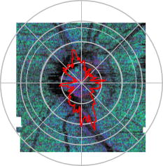 4.ConclusionsRNFL phase retardation was measured by PS-SD-OCT and GDx-VCC. In the healthy eye, both PS-SD-OCT and GDx-VCC had the double-hump pattern of RNFL. PS-SD-OCT had several peaks of the phase retardation near the retinal blood vessels. GDx-VCC also had such peaks in the en face phase retardation image, but they were smoothed in the phase retardation curve of the annular area. The DPPR/UD of the healthy eye measured by PS-SD-OCT was in the same order as the previously published results. In the glaucomatous eye, the double-hump pattern of RNFL was degraded in both PS-SD-OCT and GDx-VCC. The phase retardation curve measured by PS-SD-OCT also had several peaks near the retinal blood vessels. Both PS-SD-OCT and GDx-VCC had higher phase retardation of the inferior region than that of the superior region, which agreed with the visual field test. The thickness and DPPR/UD of the glaucomatous eye were less reliable than that of the healthy eye. To our knowledge, this is the first time PS-OCT and SLP have been compared quantitatively. Our results suggest that PS-SD-OCT can measure the cumulative phase retardation of RNFL as well as GDx-VCC. In addition, PS-SD-OCT has the ability to measure the thickness and birefringence of RNFL. Although further study is required, PS-SD-OCT can potentially be used to diagnose glaucoma by using these three parameters. AcknowledgmentsThe authors acknowledge the contribution of K. Kawana for his medical support. This project has been supported by Grants-in-Aid for Scientific Research Nos. 15760026 and 18360029 from the Japan Society for the Promotion of Science (JSPS), Japan Science and Technology Agency, and Special Research Project of Nanoscience at the University of Tsukuba. M. Yamanari has been supported in part by the Ministry of Education, Culture, Sports, Science, and Technology in Japan under the 21st Century Center of Excellence Program “Promotion of Creative Interdisciplinary Materials Science for Novel Functions.” ReferencesH. A. Quigley,
E. M. Addicks, and
W. R. Green,
“Optic nerve damage in human glaucoma. III. quantitative correlation of nerve fiber loss and visual field defect in glaucoma, ischemic neuropathy, papilledema, and toxic neuropathy,”
Arch. Ophthalmol. (Chicago), 100 135
–146
(1982). 0003-9950 Google Scholar
D. Huang,
E. A. Swanson,
C. P. Lin,
J. S. Schuman,
W. G. Stinson,
W. Chang,
M. R. Hee,
T. Flotte,
K. Gregory,
C. A. Puliafito, and
J. G. Fujimoto,
“Optical coherence tomography,”
Science, 254 1178
–1181
(1991). https://doi.org/10.1126/science.1957169 0036-8075 Google Scholar
J. S. Schuman,
M. R. Hee,
C. A. Puliafito,
C. Wong,
T. Pedut-Kloizman,
C. P. Lin,
E. Hertzmark,
J. A. Izatt,
E. A. Swanson, and
J. G. Fujimoto,
“Quantification of nerve fiber layer thickness in normal and glaucomatous eyes using optical coherence tomography,”
Arch. Ophthalmol. (Chicago), 113 586
–596
(1995). 0003-9950 Google Scholar
R. N. Weinreb,
A. W. Dreher,
A. Coleman,
H. Quigley,
B. Shaw, and
K. Reiter,
“Histopathologic validation of Fourier-ellipsometry measurements of retinal nerve fiber layer thickness,”
Arch. Ophthalmol. (Chicago), 108 557
–560
(1990). 0003-9950 Google Scholar
A. W. Dreher,
K. Reiter, and
R. N. Weinreb,
“Spatially resolved birefringence of the retinal nerve fiber layer assessed with a retinal laser ellipsometer,”
Appl. Opt., 31 3730
–3735
(1992). 0003-6935 Google Scholar
Q. Zhou and
R. N. Weinreb,
“Individualized compensation of anterior segment birefringence during scanning laser polarimetry,”
Invest. Ophthalmol. Visual Sci., 43 2221
–2228
(2002). 0146-0404 Google Scholar
M. R. Hee,
D. Huang,
E. A. Swanson, and
J. G. Fujimoto,
“Polarization-sensitive low-coherence reflectometer for birefringence characterization and ranging,”
J. Opt. Soc. Am. B, 9 903
–908
(1992). 0740-3224 Google Scholar
J. F. de Boer,
T. E. Milner,
M. J. C. van Gemert, and
J. S. Nelson,
“Two-dimensional birefringence imaging in biological tissue by polarization-sensitive optical coherence tomography,”
Opt. Lett., 22 934
–936
(1997). 0146-9592 Google Scholar
B. Cense,
T. C. Chen,
B. H. Park,
M. C. Pierce, and
J. F. de Boer,
“In vivo depth-resolved birefringence measurements of the human retinal nerve fiber layer by polarization-sensitive optical coherence tomography,”
Opt. Lett., 27 1610
–1612
(2002). https://doi.org/10.1364/OL.27.001610 0146-9592 Google Scholar
M. Pircher,
E. Götzinger,
O. Findl,
S. Michels,
W. Geitzenauer,
C. Leydolt,
U. Schmldt-Erfurth, and
C. K. Hitzenberger,
“Human macula investigated in vivo with polarization-sensitive optical coherence tomography,”
Invest. Ophthalmol. Visual Sci., 47 5487
–5494
(2006). https://doi.org/10.1167/iovs.05-1589 0146-0404 Google Scholar
R. Leitgeb,
C. K. Hitzenberger, and
A. F. Fercher,
“Performance of Fourier domain, vs. time domain optical coherence tomography,”
Opt. Express, 11 889
–894
(2003). 1094-4087 Google Scholar
J. F. de Boer,
B. Cense,
B. H. Park,
M. C. Pierce,
G. J. Tearney, and
B. E. Bouma,
“Improved signal-to-noise ratio in spectral-domain compared with time-domain optical coherence tomography,”
Opt. Lett., 28 2067
–2069
(2003). https://doi.org/10.1364/OL.28.002067 0146-9592 Google Scholar
N. Nassif,
B. Cense,
B. H. Park,
S. H. Yun,
T. C. Chen,
B. E. Bouma,
G. J. Tearney, and
J. F. de Boer,
“In vivo human retinal imaging by ultrahigh-speed spectral domain optical coherence tomography,”
Opt. Lett., 29 480
–482
(2004). https://doi.org/10.1364/OL.29.000480 0146-9592 Google Scholar
Y. Yasuno,
S. Makita,
Y. Sutoh,
M. Itoh, and
T. Yatagai,
“Birefringence imaging of human skin by polarization-sensitive spectral interferometric optical coherence tomography,”
Opt. Lett., 27 1803
–1805
(2002). https://doi.org/10.1364/OL.27.001803 0146-9592 Google Scholar
B. Cense,
“Optical coherence tomography for retinal imaging,”
Twente University,
(2005). Google Scholar
E. Götzinger,
M. Pircher, and
C. K. Hitzenberger,
“High-speed spectral domain polarization sensitive optical coherence tomography of the human retina,”
Opt. Express, 13 10217
–10229
(2005). https://doi.org/10.1364/OPEX.13.010217 1094-4087 Google Scholar
C. E. Saxer,
J. F. de Boer,
B. H. Park,
Y. Zhao,
Z. Chen, and
J. S. Nelson,
“High-speed fiber-based polarization-sensitive optical coherence tomography of in vivo human skin,”
Opt. Lett., 25 1355
–1357
(2000). https://doi.org/10.1364/OL.25.001355 0146-9592 Google Scholar
S. Jiao,
G. S. W. Yu, and
L. V. Wang,
“Optical-fiber-based Mueller optical coherence tomography,”
Opt. Lett., 28 1206
–1208
(2003). https://doi.org/10.1364/OL.28.001206 0146-9592 Google Scholar
B. H. Park,
M. C. Pierce,
B. Cense, and
J. F. de Boer,
“Jones matrix analysis for a polarization-sensitive optical coherence tomography system using fiber-optic components,”
Opt. Lett., 29 2512
–2514
(2004). https://doi.org/10.1364/OL.29.002512 0146-9592 Google Scholar
B. Cense,
T. C. Chen,
B. H. Park,
M. C. Pierce, and
J. F. de Boer,
“Thickness and birefringence of healthy retinal nerve fiber layer tissue measured with polarization-sensitive optical coherence tomography,”
Invest. Ophthalmol. Visual Sci., 45 2606
–2612
(2004). https://doi.org/10.1167/iovs.03-1160 0146-0404 Google Scholar
B. Cense,
M. Mujat,
T. C. Chen,
B. H. Park, and
J. F. de Boer,
“Polarization-sensitive spectral-domain optical coherence tomography using a single line scan camera,”
Opt. Express, 15 2421
–2431
(2007). https://doi.org/10.1364/OE.15.002421 1094-4087 Google Scholar
M. Mujat,
B. H. Park,
B. Cense,
T. C. Chen, and
J. F. de Boer,
“Autocalibration of spectral-domain optical coherence tomography spectrometers for in vivo quantitative retinal nerve fiber layer birefringence determination,”
J. Biomed. Opt., 12 041205
(2007). https://doi.org/10.1117/1.2764460 1083-3668 Google Scholar
H. Bagga,
D. S. Greenfield,
W. Feuer, and
R. W. Knighton,
“Scanning laser polarimetry with variable corneal compensation and optical coherence tomography in normal and glaucomatous eyes,”
Am. J. Ophthalmol., 135 521
–529
(2003). https://doi.org/10.1016/S0002-9394(02)02077-9 0002-9394 Google Scholar
N. J. Reus,
T. P. Colen, and
H. G. Lemij,
“Visualization of localized retinal nerve fiber layer defects with the GDx with individualized and with fixed compensation of anterior segment birefringence,”
Ophtalmologie, 110 1512
–1516
(2003). 0989-3105 Google Scholar
N. J. Reus and
H. G. Lemij,
“The relationship between standard automated perimetry and GDx VCC measurements,”
Invest. Ophthalmol. Visual Sci., 45 840
–845
(2004). https://doi.org/10.1167/iovs.03-0646 0146-0404 Google Scholar
X.-R. Huang,
H. Bagga,
D. S. Greeniedl, and
R. W. Knighton,
“Variation of peripapillary retinal nerve fiber layer birefringence in normal human subjects,”
Invest. Ophthalmol. Visual Sci., 45 3073
–3080
(2004). https://doi.org/10.1167/iovs.04-0110 0146-0404 Google Scholar
M. Wojtkowski,
V. Srinivasan,
J. G. Fujimoto,
T. Ko,
J. S. Schuman,
A. Kowalczyk, and
J. S. Duker,
“Three-dimensional retinal imaging with high-speed ultrahigh-resolution optical coherence tomography,”
Ophthalmology, 112 1734
–1746
(2005). https://doi.org/10.1016/j.ophtha.2005.05.023 0161-6420 Google Scholar
M. Yamanari,
S. Maklta,
V. D. Madjarova,
T. Yatagai, and
Y. Yasuno,
“Fiber-based polarization-sensitive Fourier domain optical coherence tomography using B-scan-oriented polarization modulation method,”
Opt. Express, 14 6502
–6515
(2006). https://doi.org/10.1364/OE.14.006502 1094-4087 Google Scholar
B. H. Park,
M. C. Pierce,
B. Cense,
S. H. Yun,
M. Mujat,
G. J. Tearney,
B. E. Bouma, and
J. F. de Boer,
“Real-time fiber-based multi-functional spectral-domain optical coherence tomography at ,”
Opt. Express, 13 3931
–3944
(2005). https://doi.org/10.1364/OPEX.13.003931 1094-4087 Google Scholar
B. Cense,
T. C. Chen,
B. H. Park,
M. C. Pierce, and
J. F. de Boer,
“In vivo birefringence and thickness measurements of the human retinal nerve fiber layer using polarization-sensitive optical coherence tomography,”
J. Biomed. Opt., 9 121
–125
(2004). https://doi.org/10.1117/1.1627774 1083-3668 Google Scholar
M. Pircher,
E. Götzinger,
R. Leitgeb,
H. Sattmann,
O. Findl, and
C. K. Hitzenberger,
“Imaging of polarization properties of human retina in vivo with phase-resolved transversal PS-OCT,”
Opt. Express, 12 5940
–5951
(2004). https://doi.org/10.1364/OPEX.12.005940 1094-4087 Google Scholar
S. Makita,
Y. Hong,
M. Yamanari,
T. Yatagai, and
Y. Yasuno,
“Optical coherence angiography,”
Opt. Express, 14 7821
–7840
(2006). https://doi.org/10.1364/OE.14.007821 1094-4087 Google Scholar
Q. Zhou,
J. Reed,
R. Betts,
P. Trost,
P.-W. Lo,
C. Wallace,
R. Bienias,
G. Li,
R. Winnick,
W. Papworth, and
M. Sinai,
“Detection of glaucomatous retinal nerve fiber layer damage by scanning laser polarimetry with variable corneal compensation,”
Proc. SPIE, 4951 32
–41
(2003). https://doi.org/10.1117/12.477975 0277-786X Google Scholar
M. Yamanari,
M. Miura,
S. Makita,
T. Yatagai, and
Y. Yasuno,
“Retinal birefringence measurement with polarization sensitive Fourier domain optical coherence tomography,”
Invest. Ophthalmol. Visual Sci., 47 3309
(2006). 0146-0404 Google Scholar
M. Yamanari,
M. Miura,
S. Makita,
T. Yatagai, and
Y. Yasuno,
“Birefringence measurement of retinal nerve fiber layer using polarization-sensitive spectral domain optical coherence tomography with Jones matrix based analysis,”
Proc. SPIE, 6429 64292M
(2007). https://doi.org/10.1117/12.702668 0277-786X Google Scholar
|


