Monte-Carlo-based model for the extraction of intrinsic fluorescence from turbid media

Gregory M. Palmer; Nirmala Ramanujam

doi:10.1117/1.2907161

1 March 2008 Monte-Carlo-based model for the extraction of intrinsic fluorescence from turbid media

Gregory M. Palmer, Nirmala Ramanujam

Author Affiliations +

Journal of Biomedical Optics, Vol. 13, Issue 2, 024017 (March 2008). https://doi.org/10.1117/1.2907161

Abstract

A Monte-Carlo-based model of fluorescence is developed that is capable of extracting the intrinsic fluorescence properties of tissue, which are independent of the absorption and scattering properties of tissue. This model is flexible in its applicability to different illumination-collection geometries and is also valid for a wide range of optical properties, representative of tissue in the UV-visible spectrum. This is potentially useful in a variety of biomedical applications, including cancer diagnostics and monitoring the physiological response to therapy. The model is validated using phantoms composed of hemoglobin (absorber), polystyrene spheres (scatterer), and furan-2 (fluorophore). It is found that this model is able to retrieve the intrinsic fluorescence spectra of the tissue phantoms and recover the intrinsic fluorescence intensity of furan within the phantoms to within a mean error of less than 10%.

1. Introduction

Fluorescence spectroscopy has been used successfully to discriminate premalignancy and malignancy in a number of organ sites.¹ However, due to the complex interplay of absorption, scattering, and fluorescence in tissue, it is difficult to separate the intrinsic fluorescence properties from absorption and scattering, thus making these spectra difficult to interpret.

To address this issue, a number of groups have proposed methods to determine the fluorophore concentration or intrinsic fluorescence spectra (i.e., the fluorescence properties independent of absorption and scattering) from a measured fluorescence spectrum. ^{2, 3, 4, 5, 6, 7, 8, 9, 10, 11, 12, 13, 14} These approaches range from empirical methods ^{2, 5, 7, 11} to diffusion theory modeling.^{3, 4} These approaches are generally limited in that they are valid for a limited range of absorption and scattering, they require extensive empirical calibration, and/or they are not flexible in their applicability to different optical probe geometries. To address these concerns a Monte-Carlo-based model to extract intrinsic tissue fluorescence is presented here. This method has the advantage that it is based on Monte Carlo modeling, and so, has the theoretical advantage of not having to impose constraints on the range of optical properties being modeled. Furthermore, this method can model the actual fiber optic probe geometry used for the fluorescence measurement and thus, in principle, is flexible in its application to a variety of probe geometries. Moreover, the approach requires only a single phantom measurement to enable adaptation to any optical system configuration (e.g., different probe geometries). This paper demonstrates its application to fluorescence spectra measured from tissue phantoms with one particular probe geometry/instrument. The companion paper¹⁵ presents the application of this model to extract intrinsic fluorescence from human breast tissue fluorescence spectra.

2. Methods

2.1.

Theory

2.1.1.

Foundation of our fluorescence model

The approach for extracting intrinsic fluorescence from a homogeneous, semiinfinite, turbid medium is achieved in two steps. First, a scalable Monte-Carlo-based model of diffuse reflectance previously developed by our group^{16, 17} is used to extract the absorption and scattering coefficients (optical properties) of the medium from a measured diffuse reflectance spectrum. Second, the optical properties are incorporated into a scalable Monte Carlo model of fluorescence to extract the intrinsic fluorescence from the raw turbid medium fluorescence. Scaling is critical to make the Monte Carlo model an efficient inversion tool for modeling tissue fluorescence.

The foundation for our fluorescence model is the work carried out previously by Swartling ¹⁸ Swartling outlined a technique wherein Monte Carlo simulations of fluorescence can be performed efficiently.¹⁸ Their approach is to break the Monte Carlo simulation into two separate simulations, one dealing with the excitation light traveling from the light source to the tissue fluorophore and one dealing with the emitted fluorescence traveling from the fluorophore to the detector. Reciprocity can also be taken advantage of to require only a single simulation for both excitation and emission. They demonstrate the use of a “reverse emission” simulation where the excitation simulation is run, and reciprocity is used to determine the emission collection probability. Each of the two baseline simulations (absorption and emission) can then be scaled to any arbitrary set of optical properties using a variety of approaches. One scaling approach that they presented was to run the baseline simulation with zero absorption, and then use Beer’s law to scale to any absorption coefficient by simply recording the path length of each photon. They also mention the possibility of a scaling approach for different scattering properties, but did not demonstrate this in their manuscript.

We have developed a fluorescence model for a semiinfinite medium, with illumination and collection at the surface of the medium, which builds on the work by Swartling ¹⁸ and Graaff ¹⁹ Figure 1 shows a flowchart of the model. Briefly, the inputs into the model are the absorption and scattering coefficient pairs of the medium at the excitation wavelengths [ $μ_{a} (λ^{x})$ , $μ_{s} (λ^{x})$ ] and emission wavelengths [ $μ_{a} (λ^{m})$ , $μ_{s} (λ^{m})$ ], the experimentally measured fluorescence spectrum $(F_{meas})$ ; and the fiber geometry collection efficiency $P (r)$ , where $r$ is the radial distance from source to exit traveled by each simulated photon. The absorption and scattering coefficients at the excitation wavelength are used to determine the absorbed energy density probability grid $A (r, z)$ , where $(r, z)$ is the point of absorption in a cylindrical coordinate system, and $A (r, z)$ gives the probability per unit volume that a photon will be absorbed at the specified coordinate. The absorption and scattering coefficients at the emission wavelength are used to determine the fluorescence escape density probability grid, $E (r, z)$ , defined as the probability per unit area that a photon originating at the coordinate $(0, z)$ ,will exit the surface of the medium at coordinate $(r, z)$ . The measured fluorescence, the absorbed energy grid, the fluorescence escape density grid, and the fiber probe geometry are incorporated into in the model to determine the intrinsic fluorescence properties of a given fluorophore, which are described by the quantum yield $(ϕ)$ , concentration $(C)$ , extinction coefficient $ε (λ)$ , and emission line shape $η (λ)$ . The intrinsic fluorescence properties are independent of the effects of absorption and scattering and the instrument configuration.

Fig. 1

Schematic showing the developed forward fluorescence model. The output of the model is shown with a bold outline, while the primary inputs are shown with a dashed outline.

While our model builds on the work by Swartling, ¹⁸ it has a few notable differences. The fluorescence escape density function grid is simulated, and reciprocity is used to determine the absorption energy density grid which is the opposite of that carried out by Swartling ¹⁸ This approach was found to yield better agreement with the original Monte Carlo simulations. Next, scaling relations described by Graaff were incorporated into this model.¹⁹ These scaling relations are used to compute the absorption and fluorescence escape density grids separately for any set of optical properties. This is performed by storing sufficient information about the path of each photon to enable its exit weight and location to be scaled to any set of optical properties. Specifically, the exit weight of each photon is given by $W_{new} = W_{sim} (a_{new} ∕ a_{sim})^{N}$ , and the exit location is given by $r_{new} = r_{sim} (μ_{t, sim} ∕ μ_{t, new})$ , where $a$ is the albedo, $W$ is the photon weight, $N$ is the number of interactions the photon underwent within the medium, $μ_{t}$ is the transport coefficient $(μ_{s} + μ_{a})$ , and $r$ is the radial distance from source to exit traveled by each photon, with the parameters specified for both the original simulation (sim) and the desired optical properties (new). These scaling relationships describe the travel of a photon between two locations in tissue. To handle differences in the anisotropy factor $g$ the scattering coefficient $μ_{s}$ was scaled such that the reduced scattering coefficient $μ_{s} (1 - g)$ was conserved, as follows, $μ_{s, new, scaled} = μ_{s, new} (1 - g_{new}) ∕ (1 - g_{sim})$ . These scaling relationships have the advantage of being able to more efficiently describe the effects of absorption outside of the diffusion regime, by taking into account the change in mean step size, which is proportional to $1 ∕ μ_{t}$ of surviving photons associated with higher absorption coefficients, as compared to a simple Beer’s law scaling, which implicitly assumes the step sizes are fixed and proportional to $1 ∕ μ_{s}$ .

The second notable difference is that the quasidiscrete Hankel transform²⁰ was used to convolve the absorption energy density and fluorescence escape function grids, enabling greater speed, which is important for clinical applications. The Hankel transform is equivalent to the 2-D Fourier transform of a circularly symmetric function. This enables convolution of the absorption energy density and fluorescence escape function simulations to be performed efficiently. We followed the approach of Li, ²⁰ who outline a computationally efficient means by which this can be performed. A third new feature of this work is that convolution was also used to model the optical probe geometry. This enables this model to be applied to any arbitrary probe configuration.

Finally, a framework was developed by which these forward simulation techniques can be applied to tissue spectra, by incorporating a scalable Monte Carlo model to calculate optical properties at both the excitation and emission wavelengths, which can then be used to solve for the intrinsic fluorescence properties of the tissue or other media independent of absorption and scattering. The fast, scalable Monte Carlo model extracts optical properties from the measured reflectance spectrum of the medium.¹⁶ The model makes it a must to know a priori what absorbers are present in the tissue and assumes that the scattering can be approximated by Mie theory scattering properties monodisperse, spherical particles.²¹ The diffuse reflectance spectrum measured from the medium is calibrated to the diffuse reflectance spectrum from a single phantom reference measurement of “known” optical properties to calibrate the system throughput and wavelength dependence. This ratio enables a direct comparison of the measured spectra to that simulated by the scalable Monte Carlo model. A nonlinear optimization algorithm is used to minimize the sum of squares error between the measured and modeled diffuse reflectance spectra by varying the absorber concentration and scatterer size/density to extract the optical properties of the medium.

2.1.2.

Implementation of the fluorescence model

First, Monte Carlo simulations were run to generate the emitted fluorescence traveling from the emitter to the detector, i.e., an escaping fluorescence energy density map $E (r, z)$ , as already defined. Photons were launched over a series of depth increments, ranging from 0 to $1 cm$ , in 0.005-cm increments, with 100,000 photons being launched at each increment. This provides an increment approximately on the order of the mean free path in tissue. A depth of $1 cm$ was chosen, since depths greater than this were found to have negligible contribution to the measured fluorescence for the probe geometry used in this study. The following parameters were used: absorption coefficient $μ_{a} = 0.01 {cm}^{- 1}$ ; scattering coefficient $μ_{s} = 150 {cm}^{- 1}$ ; anisotropy factor $g = 0.8$ ; refractive index of medium; 1.335 (corresponds to that of the phantoms); and refractive index of fused silica fiber; 1.47. Photons that escape to the surface of the medium and which are within the numerical aperture (NA) of the detector fiber (in our case, the NA is 0.12) were stored in an array, containing the exit weight, launch depth $(z)$ , net radial distance traveled $(r)$ , and number of interactions $(N)$ within the medium prior to escape.

Next, using the principle of reciprocity, it is possible to determine the course of the excitation light traveling from the light source to the tissue fluorophore, i.e., how much light energy would be absorbed at a given location within the medium were the photon launched at the surface of the tissue using a fiber with the same NA. However, note that one must account for the difference in solid angle between the acceptance/emission of light by the absorber/fluorophore within the tissue $(4 π)$ and the limited acceptance angle of the source/detector fiber (defined by the NA). The acceptance/emission solid angle for a single molecule would not be $4 π$ , but for a suspension of randomly oriented molecules, the collective acceptance/emission is uniform. Swartling derived the effect of a difference in solid angle between the source and detector and the acceptance/emission of light by the absorbers/fluorophores,¹⁸ and using this factor $(4 π ∕ Δ Ω)$ , the relationship between $E (r, z)$ and $A (r, z)$ is given by

Eq. 1

A (r, z) = \frac{4 π}{Δ Ω} μ_{a} (λ^{x}) E (r, z),

where

A (r, z)

is the absorbed energy density (already defined);

Δ Ω

is the solid angle corresponding to the fiber’s NA, given by

Δ Ω = 2 π {1 - \cos [\sin^{- 1} (NA ∕ n_{medium})]}

;

n_{medium}

is the refractive index of the turbid medium or tissue; and

μ_{a} (λ^{x})

is the absorption coefficient at the excitation wavelength. This relationship makes it possible to require only a single set of simulations to generate both the fluorescence escape function and absorbed energy density grids. Note that

E (r, z)

is dependent on both the absorption and scattering properties of the medium at the emission wavelength. The additional dependence on absorption,

μ_{a}^{x}

in Eq. 1 converts fluence to absorption. Since the exiting location of each photon can be stored exactly, it also enables the elimination of a fixed radial grid, which can lead to inaccuracies at short source detector separations due to interpolation/extrapolation of the spatial grid. The previously described scaling relations can then be used to scale the absorption grid and the fluorescence escape function grid for the desired optical properties.

Not all of the absorbed energy is converted to fluorescence. The probability of an absorbed photon generating a fluorescent photon at a given emission wavelength is given by Swartling ¹⁸ as

Eq. 2

ϕ_{eff} (λ^{x}, λ^{m}) = ϕ \frac{μ_{a}^{f} (λ^{x})}{μ_{a} (λ^{x})} \frac{η (λ^{m}) Δ λ^{m}}{\int_{0}^{\infty} η (λ^{m}) d λ^{m}},

where

ϕ_{eff}

is the effective quantum yield for a given excitation

(λ^{x})

emission

(λ^{m})

wavelength pair in the medium of interest,

ϕ

is the fluorescence quantum yield,

μ_{a}^{f} (λ^{x})

is the absorption coefficient of the fluorophore at the excitation wavelength,

μ_{a} (λ^{x})

is the total absorption coefficient of all absorbers in the medium at the excitation wavelength, and

η (λ^{m})

is the spectral probability distribution of the generated fluorescence as a function of the emission wavelength. This equation thus takes into account the probability that a photon absorbed by the fluorophore will generate fluorescence

(ϕ)

, the probability that an absorbed photon will be absorbed by the fluorophore rather than another absorber

[μ_{a}^{f} (λ^{x}) ∕ μ_{a} (λ^{x})]

, and the probability that a generated fluorescent photon will be emitted at the collected emission wavelength (the remaining terms). These fluorescence parameters are the output of the model, and so this is not actually calculated, as will be developed below.

Given $A (r, z)$ and Eq. 2, it is then possible to determine the generated fluorescence energy density at all points within the medium for any given set of optical properties at the excitation wavelength and for a given set of fluorescence properties [ $ϕ$ , $μ_{a}^{f} (λ^{x})$ , $η (λ^{m})$ ] as follows:

Eq. 3

F_{gen} (r, z) = ϕ_{eff} (λ^{x}, λ^{m}) A (r, z),

where

F_{gen} (r, z)

is the fluorescence energy density generated within the medium as a function of depth

z

and radial distance

r

. The fluorescence generated at a given depth is then convolved with the fluorescence escape energy density to obtain the exit probability of fluorescent photons escaping the surface of the medium to be collected. Summing over the entire range of depths within the medium gives the total emitted fluorescence as a function of radial distance. Thus, the emitted fluorescence is given by

Eq. 4

F_{exit} (r) = \sum_{j} Δ z_{j} F_{gen} (r, z_{j}) * E (r, z_{j}),

where

F_{exit} (r)

is the radially dependent fluorescence exiting the surface of the tissue, and

Δ z

gives the grid size in the depth dimension for each summed grid element. This could also be expressed as an integral, but we chose to express it as a discrete sum since this is what was done in practice.

The inverse problem is solved by noting that since $ϕ_{eff}$ is a scalar, owing to the associative property of convolution, substituting Eq. 3 into Eq. 4, it can be taken out of the summation in Eq. 4, as

Eq. 5

F_{exit} (r) = ϕ_{eff} (λ^{x}, λ^{m}) \sum_{j} Δ z_{j} A (r, z_{j}) * E (r, z_{j}) .

The terms within the summation depend on only the optical properties of the medium at the excitation and emission wavelengths, and not on the fluorescence properties of the medium. In particular, $A (r, z)$ is a function of the optical properties at the excitation wavelength, and $E (r, z)$ is a function of the optical properties at the emission wavelength. Furthermore, note that in Eq. 2, for a known fluorophore, the wavelength-dependent extinction coefficients and emission spectra are known. Thus, $ϕ_{eff} (λ^{x}, λ^{m})$ can be expressed as the product of the fluorophore concentration, the quantum yield, and a set of wavelength dependent constants, as

Eq. 6

ϕ_{eff} (λ^{x}, λ^{m}) = ϕ \frac{μ_{a}^{f} (λ^{x})}{μ_{a} (λ^{x})} \frac{η (λ^{m}) Δ λ}{\int_{0}^{\infty} η (λ^{m}) d λ} = ϕ \frac{2.303 ε (λ^{x}) C}{μ_{a} (λ^{x})} \frac{η (λ^{m}) Δ λ^{m}}{\int_{0}^{\infty} η (λ^{m}) d λ^{m}},

where

C

is the fluorophore concentration, and

ε (λ^{x})

is the extinction coefficient of the fluorophore at the excitation wavelength.

Because $E (r, z)$ , and hence $A (r, z)$ , were simulated using a point source, the convolution of the two terms results in the radial distribution of fluorescence occurring using a point source illumination. To account for the probe, one must then multiply this with the probe specific collection probability as a function of radial distance and sum over all distances. The collection probability for a probe geometry consisting of separate illumination and collection fibers is given in Refs. 16, 22 (note errata²² to original manuscript¹⁶) as

Eq. 7

P (r) = \frac{2}{π^{2} R_{i}^{2}} \int_{\max (- R_{i}, s - r - R_{c})}^{\min (R_{i}, s - r + R_{c})} (s - x) \cos^{- 1} [\frac{s^{2} + {(s - x)}^{2} - R_{i}^{2}}{2 (s - x) s}] \cos^{- 1} [\frac{r^{2} + {(s - x)}^{2} - R_{c}^{2}}{2 (s - x) r}] d x,

where

P (r)

is the probability that a photon traveling a distance

r

will be collected given two separate source-detector fibers;

R_{i}

and

R_{c}

are the radii of these illumination and detection fibers, respectively;

s

is the center-center separation of these fibers; and

x

is the spatial variable corresponding to launch locations across the face of the illumination fiber over which the integration is performed. These parameters were obtained by imaging our fiber optic probe using a reflected-light microscope and applying this formula to all fibers, pairwise. Note that a fiber-optic-based measurement was utilized in this implementation, but the theory involved is applicable to imaging systems as well. Incorporating the specific probe geometry used, and combining Eqs. 5, 6, we get

Eq. 8

F_{meas} (λ^{x}, λ^{m}) = S ϕ \frac{2.303 C ε (λ^{x})}{μ_{a} (λ^{x})} \frac{η (λ^{m}) Δ λ^{m}}{\int_{0}^{\infty} η (λ^{m}) d λ^{m}} \sum_{i} {a_{i} P (r_{i}) \sum_{j} [Δ z_{j} A (r_{i}, z_{j}) * E (r_{i}, z_{j})]},

or

Eq. 9

2.303 C ε (λ^{x}) ϕ \frac{η (λ^{m}) Δ λ^{m}}{\int_{0}^{\infty} η (λ^{m}) d λ^{m}} = \frac{μ_{a} (λ^{x}) F_{meas} (λ^{x}, λ^{m})}{S \sum_{i} {a_{i} P (r_{i}) \sum_{j} [Δ z_{j} A (r_{i}, z_{j}) * E (r_{i}, z_{j})]}} .

$a_{i}$ is the surface area of each radial grid element. Just to clarify, all of the parentheses indicate functional relationships or summations, and are not products. Also $F_{meas} (λ^{x}, λ^{m})$ is the fluorescence measured using a particular probe geometry, given the optical $[μ_{a} (λ^{x}, λ^{m}), μ_{s}^{'} (λ^{x}, λ^{m})]$ and fluorescence properties $[ϕ, ε (λ^{x}), η (λ^{m}), C]$ of the medium, and $S$ is introduced here as a scaling factor necessary to account for the difference in magnitude between the Monte Carlo simulations, which are on an absolute scale, and the measurement, which is typically relative to a fluorescence standard. This factor must be determined using a phantom measurement to pool data collected using different instruments or probe geometries. For a single instrument setup, it can be set to unity to leave the intrinsic fluorescence spectra on a relative scale. The quantum yields, extinction coefficients, and emission efficiencies could be independently determined, allowing an absolute determination of fluorophore concentration in tissue. The result of this model thus allows for the extraction of intrinsic fluorescence line shape, and intensity, independent of the effects of absorption and scattering. This quantity is proportional to the product of the concentration and fluorescence quantum yield. This can in turn be used to determine the product of the fluorophore concentration provided that some a priori information is known about the fluorophore.

2.2.

Phantom Validation

The model just described was tested using synthetic liquid tissue phantoms. Liquid phantoms were made using hemoglobin (H0267, Sigma-Aldrich Corp.) as the absorber, furan-2 as the fluorophore, and polystyrene spheres (07310, Polysciences, Inc.) as the scatterer. Three sets of phantoms were prepared, having low, medium, and high scattering properties. Into each phantom, $12 μ g ∕ ml$ of furan-2 was added (which contributes negligible absorption), and varying concentrations of hemoglobin were added in to change the absorption properties of the medium, yielding a total of 11 phantoms. One phantom was an outlier, having significantly lower (25 to 50%) fluorescence and reflectance intensity relative to the other phantoms (likely due to incomplete probe contact) and was excluded. The absorption coefficient of hemoglobin was determined using a spectrophotometer (Cary 300, Varian, Inc.), and the scattering coefficient of the polystyrene spheres was calculated using Mie theory,^{21, 23} taking into account the wavelength dependent real refractive index of polystyrene spheres²⁴ and water.²⁵ Both the spheres and water were assumed to be nonabsorbing in the analysis, although the effects of absorption by spheres were evaluated separately. Table 1 summarizes the optical properties of the phantoms over the wavelength range of 330 to $600 nm$ . Phantoms 1 to 4 correspond to low scattering, 5 to 8 correspond to medium scattering, and 9 to 11 correspond to high scattering. Within each scattering level, as the phantom number increases, more hemoglobin has been added, so the absorption coefficients increase, while the scatterer is diluted slightly, so the scattering coefficients decrease. These phantoms are designed to mimic tissue optical properties in the UV to visible spectral range, and specifically correspond to the optical properties we have observed in breast tissues.¹⁷ Phantom 6 was used as the reference phantom for the purposes of extracting the optical properties of all phantoms because it is in the middle of the range for both absorption and scattering.

Table 1

Summary of the optical properties of the phantoms used to validate the fluorescence model over the wavelength range of 330 to 600nm .

	Absorption Coefficient μa				Reduced Scattering Coefficient μs′
Phantom Number	Min (cm−1)	Max (cm1)	Mean (cm−1)	Mean Relative Error of Extraction (%)	Min (cm1)	Max (cm1)	Mean (cm1)	Mean Relative Error of Extraction (%)
1	0.0	0.9	0.2	26.1	3.9	5.9	4.6	4.9
2	0.1	6.8	1.4	24.9	3.8	5.8	4.5	8.0
3	0.1	12.4	2.6	27.1	3.7	5.7	4.4	12.3
4	0.2	22.9	4.8	26.5	3.6	5.4	4.2	16.1
5	0.0	0.9	0.2	11.9	11.7	17.7	13.9	0.8
6	0.0	6.8	1.4	0.0	11.4	17.3	13.5	0.0
7	0.0	12.4	2.6	4.4	11.2	16.9	13.2	1.9
8	0.0	22.9	4.8	5.8	10.7	16.1	12.6	3.2
9	0.0	6.7	1.4	7.0	19.0	28.7	22.4	18.8
10	0.0	12.3	2.6	1.2	18.5	28.1	21.9	18.8
11	0.0	22.7	4.8	2.4	17.7	26.8	21.0	16.7

Phantoms 1 to 4 correspond to low scattering, 5 to 8 correspond to medium scattering, and 9 to 11 correspond to high scattering. Also shown are the mean relative errors in the optical property extraction using the diffuse reflectance model.

The SkinSkan fluorometer (J.Y. Horiba) and fiber optic probe were used for making all experimental diffuse reflectance and fluorescence measurements from the synthetic liquid tissue phantoms. Briefly, the instrument consists of a 150-W xenon lamp, dual excitation and emission grating monochromators, and a photomultiplier tube (PMT) detector. Diffuse reflectance measurements were collected using a “synchronous scan,” wherein the excitation and emission monochromators are scanned in tandem across the wavelength range of interest (330 to $600 nm$ ). Fluorescence emission spectra were acquired by fixing the excitation monochromator to $330 nm$ and scanning the emission monochromator from 350 to $500 nm$ . All scans were run with a 5-nm increment. The fiber optic probe consisted of a central collection core with a diameter of $1.52 mm$ , surrounded by an illumination ring with an outer diameter of $2.18 mm$ . Both the illumination core and surrounding ring consisted of 31 fibers, each of which had a core/cladding diameter of $200 ∕ 245 μ m$ .

The diffuse reflectance (330 to $600 nm$ ) and fluorescence (330-nm excitation) were measured from each sample by placing the probe submerged just below the surface of the phantom. The tip of the probe was sealed with epoxy between the fibers, preventing any capillary action. Each phantom was placed in a container of approximately 1.5-cm diameter, with a total volume of $8 ml$ , which satisfied the criterion of a semiinfinite medium for the model. This was tested by measuring with the probe at the surface of the medium, and submerged halfway down, with no observable difference in the signal intensities. Then the scalable Monte Carlo model was used to extract the optical properties of each sample from the measured diffuse reflectance using procedures described in Ref. 16. The extracted optical properties were input to the fluorescence model to retrieve the intrinsic fluorescence from the measured phantom fluorescence. In addition, the “known” optical properties, taken from Mie theory and the spectrophotometer measurement, were also used as inputs into the fluorescence model to retrieve the intrinsic fluorescence. This allows for an assessment of the propagation of errors from the reflectance model to the fluorescence model. To illustrate the effectiveness of the model in determining the intrinsic fluorescence properties within the medium, Eq. 9 was solved for the product:

Eq. 10

ϕ \frac{η (λ^{m}) Δ λ^{m}}{\int_{0}^{\infty} η (λ^{m}) d λ^{m}} .

The concentration (which is known) was divided out in Eq. 10 since it was diluted slightly with increasing absorber concentration. This is done since otherwise the magnitude of the intrinsic fluorescence would vary with concentration. Dividing this out enables an evaluation of the variability in the data associated with the model/experimental errors only, independent of the concentration of the fluorophore. Assuming that the quantum yield

ϕ

is constant in each of the phantoms, this quantity plotted as a function of wavelength demonstrates the ability of this method to retrieve the intrinsic fluorescence line shape and intensity. The ideal result would yield overlapping curves for each of the phantoms, with identical intensities and line shapes that match that of furan fluorescence. The degree to which these quantities deviate from each other indicates the errors that would be obtained in calculating the intrinsic fluorescence. In this paper, relative errors in extraction of intrinsic fluorescence intensity are reported, using the mean intrinsic fluorescence intensity of all phantoms taken as the desired value. Since only a single probe and instrument were used,

S

was set to unity for simplicity. For the case of the analysis using the extracted optical properties, the “true” intrinsic fluorescence was taken as the mean of that obtained using the “known” optical properties of the set of phantoms, to enable an evaluation of the propagation of errors from the reflectance to the fluorescence models.

3. Results

Table 1 shows the extraction errors for each of the phantom’s optical properties, as compared to the expected values. Phantom 6, a middle-level scatterer, was used as the reference phantom for the extraction, hence it has low errors, as do the phantoms with similar optical properties. The low- and high-scattering phantoms each show larger errors, relative to the middle-scattering level. There are relatively smaller increases in the extraction errors as the absorption coefficient is varied for the same scatterer level. This indicates that varying the density of polystyrene spheres causes larger deviations in the extracted optical properties than does varying the absorber concentration. This may be attributed to uncertainty in the optical properties of polystyrene spheres, as discussed further in the following.

Figure 2 shows the product in Eq. 10 for the nonnormalized [Figs. 2a, 2b, 2c] and normalized [Figs. 2d, 2e, 2f] fluorescence spectra, acquired at 330-nm excitation. The nonnormalized spectra plots, shows the raw fluorescence spectra [Fig. 2a], intrinsic fluorescence using the extracted optical properties [Fig. 2b], and intrinsic fluorescence using the “known” optical properties [Fig. 2c]. The normalized plots show the same data sets in Figs. 2d, 2e, 2f], respectively, normalized to their peak intensity. The fluorescence spectral line shape acquired with no absorber or scatterer present is also shown in the normalized plots (black line) and can be seen to be very similar to the extracted line shape for the cases where the known, and extracted optical properties were used. We can see that the model corrects for the original large differences in magnitude and line shape present due to the differences in absorption and scattering in each of the phantoms.

Fig. 2

(a) to (c) Nonnormalized and (d) to (f) normalized fluorescence spectra, acquired at 330-nm excitation. The nonnormalized spectra plots, shows the (a) raw fluorescence spectra, (b) intrinsic fluorescence using the extracted optical properties, and (c) intrinsic fluorescence using the “known” optical properties. The normalized plots show the same data sets (d), (e), and (f), respectively, normalized to their peak intensity. The fluorescence spectral line shape acquired with no absorber or scatterer present is also shown in the normalized plots (black line) and can be seen to be very similar to the extracted line shape for the cases were the known and extracted optical properties were used. Phantoms with the same color have the same absorber concentration (higher absorption having lower reflectance), while phantoms having the same line style have the same scatterer concentration (solid, low; dashed, medium; dotted, high). The legend indicates the phantom number (see Table 1).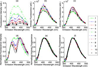

Table 2 quantifies the errors in line shape and intensity extracted for the 11 phantoms. Line shape was evaluated by calculating the fraction of variance accounted for by the line shape of the fluorophore that is measured in a dilute solution (this provides the known intrinsic line shape), using a linear fit. This is given by the relationship 1-SSE/SST, where SSE is the sum of squares of the residuals in this fit, and SST is the sum of squares of the original spectra. This represents the $R^{2}$ values, all of which are above 0.98. The percent deviation from the mean peak intrinsic fluorescence intensity of furan for all phantoms [determined from Eq. 10] was $9.3 \pm 9.8 %$ for the case where the optical properties were extracted from the diffuse reflectance and $9.1 \pm 4.7 %$ where the known optical properties were used. The phantoms with the lowest scattering properties (1 to 4) appear to have generally higher errors than the more scattering phantoms. This is significant for the use of known optical properties ( $p < 0.001$ using a $t$ test), but not significant for the use of extracted optical properties.

Table 2

The variance of the intrinsic line shape is well described by the fluorescence spectrum of furan-2 in a dilute solution, as indicated by high R2 values; and the percent deviations from the mean intensity for each of the phantoms.

Phantom	Line Shape—Extracted Optical Properties (R2)	Line Shape—Known Optical Properties (R2)	Deviation in Intensity—Extracted Optical Properties (%)	Deviation in Intensity—Known Optical Properties (%)
1	0.99	0.99	$- 23.8$	$- 13.5$
2	0.98	0.99	$- 12.8$	12.0
3	0.98	0.99	$- 18.4$	16.0
4	0.98	0.98	$- 27.0$	12.3
5	0.99	0.99	$- 8.1$	$- 12.3$
6	0.99	0.99	0.2	0.2
7	0.99	0.99	$- 1.2$	3.4
8	0.99	0.99	$- 2.3$	6.1
9	1.00	1.00	5.8	$- 8.7$
10	1.00	1.00	0.3	$- 7.5$
11	0.99	1.00	$- 2.7$	$- 8.0$

Following up on this finding, we evaluated the effects of the assumption that the polystyrene spheres contribute negligible absorption to the phantoms. There are no data to our knowledge characterizing the complex refractive index of polystyrene spheres at UV wavelengths down to $330 nm$ . However, using the findings of Ma ²⁴ as a guide, we experimented with two different imaginary components of the refractive index, $- 0.0004$ , which is approximately the value Ma reported throughout the visible,²⁴ and $- 0.0001$ , which corresponds to lower absorption, which was arbitrarily chosen. Table 3 shows the results of using these imaginary components in calculation of the absorption and scattering properties of these phantoms. We can see that the incorporation of absorption by the spheres substantially improves the accuracy with which the intrinsic fluorescence intensity can be extracted for the “known” optical properties, but not in the case of the extracted optical properties. This may be due to the inverse problem becoming more poorly conditioned when the concentration of polystyrene spheres affects both the absorption and scattering properties, resulting in greater errors in the extracted optical properties. Interestingly, using the imaginary component at only the excitation wavelength results in similar error reduction as the case where it is used at both the excitation and emission wavelengths.

Table 3

Mean relative error of the extracted fluorescence intensity using the “known” and extracted optical properties.

Imaginary Refractive Index of Polystyrene Spheres	Mean Relative Error Using “Known” Optical Properties	Mean Relative Error Using Extracted Optical Properties
0 (nonabsorbing)	$9.1 \pm 4.7 %$	$9.3 \pm 9.8 %$
$- 0.0001$ at all $λ$	$7.0 \pm 4.0 %$	$10.5 \pm 10.8 %$
$- 0.0004$ at all $λ$	$4.5 \pm 4.7 %$	$15.7 \pm 12.6 %$
$- 0.0001$ at excitation only	$7.7 \pm 4.2 %$	$10.0 \pm 10.2 %$
$- 0.0004$ at excitation only	$4.4 \pm 4.1 %$	$12.8 \pm 11.4 %$
$- 0.0001$ at emission only	$8.5 \pm 4.5 %$	$9.7 \pm 10.3 %$
$- 0.0004$ at emission only	$6.5 \pm 4.1 %$	$11.4 \pm 11.3 %$

The inclusion of absorption by polystyrene spheres through the imaginary component of the refractive index substantially improves the accuracy when using known optical properties, but not the measured optical properties.

4. Discussion

This paper outlined a methodology by which intrinsic fluorescence spectra can be extracted from combined fluorescence and diffuse reflectance spectra, which are commonly measured from tissues in a variety of clinical and preclinical studies. This enables more biologically relevant interpretation of these data, since they can be directly related to underlying tissue properties (fluorophore concentrations or microenvironment). The significant advantages of this model are (1) it does not require any assumptions regarding the underlying fluorescence properties in order to calculate the intrinsic fluorescence spectra; (2) it is able to account for any arbitrary probe geometry; (3) it does not require extensive empirical calibration; (4) it is appropriate to use for cases of high absorption and small source-detector separation; and (5) since the intrinsic fluorescence properties are instrument independent, it allows for data acquired from multiple instruments and/or probe geometries to be pooled. This pooling would require the use of a phantom measurement to determine the instrument dependent factor $S$ , as already described, or in lieu of that, the data could be normalized and pooled on a relative scale to eliminate this requirement. This model can be used to extract endogenous sources of fluorescence as well as characterize the prevalence of exogenous sources of fluorescence in turbid media.

The application of this model to phantoms was relatively straightforward, since all of the constituents were known and well characterized, and reasonably good accuracy was obtained in extracting the intrinsic fluorescence line shape and intensity. This model performs well for the entire range of optical properties tested. A significant source of error appears to relate to the accuracy with which the optical properties of polystyrene spheres are quantified. This is reflected by the fact the intrinsic fluorescence intensity extraction accuracy was highly sensitive to the imaginary refractive index of polystyrene used in the model (see Table 3). Unfortunately, there is limited information on the optical properties of polystyrene spheres, and these optical properties may vary depending on the source, since absorption is likely highly influenced by contaminants (see Ref. 26 for a detailed discussion). There is no information to our knowledge reporting the optical properties of polystyrene spheres at the excitation wavelength of $330 nm$ , so it was necessary to extrapolate the findings of Ma ²⁴ It was found that using an imaginary refractive index of $1 e - 4$ , substantially reduced the errors in the extracted intrinsic fluorescence intensity from $9.1 \pm 4.7$ down to $4.5 \pm 4.7$ (see Table 3). It appears that the errors found in the model are most highly influenced by the optical properties at the excitation wavelength. Using the complex refractive index at the excitation wavelength alone, produced the same reduction in error as using it over the entire wavelength range. It is also possible that the real component of the refractive index is inaccurate at the excitation wavelength, as we had to employ extrapolation here as well. Any such analysis is rather speculative, but serves to point out potential sources of error.

Another potential source of error is the fact that the Henyey-Greenstein phase function was used in the Monte Carlo simulations, rather than the Mie phase function. The robustness of this model is well demonstrated by the fact that, despite these uncertainties, in the simplest case of nonabsorbing spheres, the model was found to be able to extract the intrinsic fluorescence intensity with mean percent errors of $9.1 \pm 4.7 %$ using the “known” optical properties, and $9.3 \pm 9.8 %$ using the extracted optical properties, thus demonstrating the usefulness of this model for a wide range of optical properties. Errors are reported in terms of the variability of the intensity of the intrinsic fluorescence. However, note that if the quantum yield, extinction coefficient, and emission spectrum could be accurately determined, or could be assumed to be constant, equivalent relative errors would be obtained in extracting the concentration of the fluorophore.

Limitations of this model include the fact that it assumes a homogeneous distribution of fluorophores with homogeneous optical properties. However, it is possible to adapt this approach to accommodate a nonhomogeneous distribution, particularly for layered media. This model as implemented also requires knowledge of the absorbers and scatterers present in the medium to retrieve the absorption and scattering properties of the medium, although other techniques for optical property retrieval could be used for this purpose that do not impose such a limitation.²⁷ This model could also be made computationally more efficient by running only a single simulation similar to the “reverse emission” approach outlined by Swartling ¹⁸ (described in the methods section of this manuscript) that could also record information required for the diffuse reflectance baseline simulation, simply by also recording photons exiting the medium.

In the companion manuscript we will explore the application of this model to fluorescence spectra measured from human breast tissues.¹⁵ Application to tissue is more challenging due to the presence of multiple absorbers, scatterers, and fluorophores of uncertain properties. However, we have previously applied the scalable Monte Carlo reflectance model to extract optical properties from breast tissue diffuse reflectance spectra,¹⁷ and the addition of the fluorescence model is relatively straightforward since it does not require any assumptions regarding the properties of the fluorophores in order to retrieve the intrinsic fluorescence. The intrinsic fluorescence defined by Eq. 10 was calculated, taking $S$ to be unity. This enables comparison of relative fluorescence intensities in tissue, where absolute calibration would be extremely difficult due to differences in microenvironment etc. that may affect fluorescence properties. In addition, the presence of multiple fluorophores requires that one separate the influence of each fluorophore spectrally. In the companion paper, multivariate curve resolution²⁸ was utilized to achieve this. It may be desirable to obtain the actual concentration of the fluorophore in future applications. However, this does require some additional knowledge of the fluorophore properties that steady state fluorescence measurements alone cannot provide, particularly the quantum yield.

Acknowledgments

This work was funded by University of Wisconsin Radiological Sciences Training Grant No. 5T32CA009206-27, sponsored by the National Institutes of Health, the Department of Health and Human Services, and the Public Health Service. Additional funding was provided by the National Institutes of Health through Grant No. 1R01CA100559-01A1 and the Department of Defense Breast Cancer Research Program Grant No. DAMD17-02-1-0628.

References

1.

N. Ramanujam, “Fluorescence spectroscopy in vivo,” Encyclopedia of Analytical Chemistry, 20 –56 John Wiley and Sons, Ltd.(2000). Google Scholar

2.

N. C. Biswal, S. Gupta, N. Ghosh, and A. Pradhan, “Recovery of turbidity free fluorescence from measured fluorescence: an experimental approach,” Opt. Express, 11 3320 –3331 (2003). 1094-4087 Google Scholar

3.

S. K. Chang, N. Marin, M. Follen, and R. Richards-Kortum, “Model-based analysis of clinical fluorescence spectroscopy for in vivo detection of cervical intraepithelial dysplasia,” J. Biomed. Opt., 11 024008 (2006). https://doi.org/10.1117/1.2187979 1083-3668 Google Scholar

4.

K. R. Diamond, T. J. Farrell, and M. S. Patterson, “Measurement of fluorophore concentrations and fluorescence quantum yield in tissue-simulating phantoms using three diffusion models of steady-state spatially resolved fluorescence,” Phys. Med. Biol., 48 4135 –4149 (2003). https://doi.org/10.1088/0031-9155/48/24/011 0031-9155 Google Scholar

5.

K. R. Diamond, M. S. Patterson, and T. J. Farrell, “Quantification of fluorophore concentration in tissue-simulating media by fluorescence measurements with a single optical fiber,” Appl. Opt., 42 2436 –2442 (2003). https://doi.org/10.1364/AO.42.002436 0003-6935 Google Scholar

6.

A. J. Durkin, S. Jaikumar, N. Ramanujam, and R. Richards-Kortum, “Relation between fluorescence spectra of dilute and turbid samples,” Appl. Opt., 33 414 –423 (1994). 0003-6935 Google Scholar

7.

C. M. Gardner, S. L. Jacques, and A. J. Welch, “Fluorescence spectroscopy of tissue: recovery of intrinsic fluorescence from measured fluorescence,” Appl. Opt., 35 1780 –1792 (1996). 0003-6935 Google Scholar

8.

M. G. Muller, I. Georgakoudi, Z. Qingguo, W. Jun, and M. S. Feld, “Intrinsic fluorescence spectroscopy in turbid media: disentangling effects of scattering and absorption,” Appl. Opt., 40 4633 –4646 (2001). https://doi.org/10.1364/AO.40.004633 0003-6935 Google Scholar

9.

Q. Zhang, M. G. Muller, J. Wu, and M. S. Feld, “Turbidity-free fluorescence spectroscopy of biological tissue,” Opt. Lett., 25 1451 –1453 (2000). 0146-9592 Google Scholar

10.

M. Sinaasappel and H. J. C. M. Sterenborg, “Quantification of the hematoporphyrin derivative by fluorescence measurement using dual-wavelength excitation and dual-wavelength detection,” Appl. Opt., 32 541 –548 (1993). 0003-6935 Google Scholar

11.

R. Weersink, M. S. Patterson, K. Diamond, S. Silver, and N. Padgett, “Noninvasive measurement of fluorophore concentration in turbid media with a simple fluorescence/reflectance ratio technique,” Appl. Opt., 40 6389 –6395 (2001). https://doi.org/10.1364/AO.40.006389 0003-6935 Google Scholar

12.

J. Wu, M. S. Feld, and R. P. Rava, “Analytical model for extracting intrinsic fluorescence in turbid media,” Appl. Opt., 32 3585 –3595 (1993). 0003-6935 Google Scholar

13.

N. N. Zhadin and R. R. Alfano, “Correction of the internal absorption effect in fluorescence emission and excitation spectra from absorbing and highly scattering media: theory and experiment,” J. Biomed. Opt., 3 171 –186 (1998). https://doi.org/10.1117/1.429874 1083-3668 Google Scholar

14.

B. W. Pogue and G. Burke, “Fiber-optic bundle design for quantitative fluorescence measurement from tissue,” Appl. Opt., 37 7429 –7436 (1998). 0003-6935 Google Scholar

15.

C. Zhu, G. M. Palmer, T. M. Breslin, J. Harter, and N. Ramanujam, “Diagnosis of breast cancer using fluorescence and diffuse reflectance spectroscopy: a Monte Carlo model based approach,” Google Scholar

16.

G. M. Palmer and N. Ramanujam, “Monte Carlo-based inverse model for calculating tissue optical properties. Part I: Theory and validation on synthetic phantoms,” Appl. Opt., 45 1062 –1071 (2006). https://doi.org/10.1364/AO.45.001062 0003-6935 Google Scholar

17.

G. M. Palmer, C. Zhu, T. M. Breslin, F. Xu, K. W. Gilchrist, and N. Ramanujam, “Monte Carlo-based inverse model for calculating tissue optical properties. Part II: Application to breast cancer diagnosis,” Appl. Opt., 45 1072 –1078 (2006). https://doi.org/10.1364/AO.45.001072 0003-6935 Google Scholar

18.

J. Swartling, A. Pifferi, A. M. Enejder, and S. Andersson-Engels, “Accelerated Monte Carlo models to simulate fluorescence spectra from layered tissues,” J. Opt. Soc. Am. A Opt. Image Sci. Vis, 20 714 –727 (2003). 1084-7529 Google Scholar

19.

R. Graaff, M. H. Koelink, F. F. M. de Mul, W. G. Zijlstra, A. C. M. Dassel, and J. G. Aarnoudse, “Condensed Monte Carlo simulations for the description of light transport [biological tissue],” Appl. Opt., 32 426 –434 (1993). 0003-6935 Google Scholar

20.

Y. Li, H. Meichun, C. Mouzhi, C. Wenzhong, H. Wenda, and Z. Zhizhong, “Quasi-discrete Hankel transform,” Opt. Lett., 23 409 –411 (1998). 0146-9592 Google Scholar

21.

C. F. Bohren and D. R. Huffman, Absorption and Scattering of Light by Small Particles, Wiley, New York (1983). Google Scholar

22.

G. M. Palmer and N. Ramanujam, “Monte Carlo-based inverse model for calculating tissue optical properties. Part I: Theory and validation on synthetic phantoms: errata,” Appl. Opt., 46 6847 (2007). https://doi.org/10.1364/AO.46.006847 0003-6935 Google Scholar

23.

S. Prahl, “Mie scattering program,” (2003) http://omlc.ogi.edu/software/mie Google Scholar

24.

X. Ma, J. Q. Lu, R. S. Brock, K. M. Jacobs, P. Yang, and X. H. Hu, “Determination of complex refractive index of polystyrene microspheres from 370 to

1610 nm

,” Phys. Med. Biol., 48 4165 –4172 (2003). https://doi.org/10.1088/0031-9155/48/24/013 0031-9155 Google Scholar

25.

, “Release on the Refractive Index of Ordinary Water Substance as a Function of Wavelength, Temperature, and Pressure,” (1997) http://www.iapws.org/relguide/rindex.pdf Google Scholar

26.

D. Passos, J. C. Hebden, P. N. Pinto, and R. Guerra, “Tissue phantom for optical diagnostics based on a suspension of microspheres with a fractal size distribution,” J. Biomed. Opt., 10 064036 (2005). https://doi.org/10.1117/1.2139971 1083-3668 Google Scholar

27.

G. M. Palmer and N. Ramanujam, “Use of genetic algorithms to optimize fiber optic probe design for the extraction of tissue optical properties,” IEEE Trans. Biomed. Eng., 54 1533 –1535 (2007). https://doi.org/10.1109/TBME.2006.889779 0018-9294 Google Scholar

28.

A. de Juan and R. Tauler, “Chemometrics applied to unravel multicomponent processes and mixtures: Revisiting latest trends in multivariate resolution,” Anal. Chim. Acta, 500 195 –210 (2003). https://doi.org/10.1016/S0003-2670(03)00724-4 0003-2670 Google Scholar

Citation Download Citation

Gregory M. Palmer and Nirmala Ramanujam "Monte-Carlo-based model for the extraction of intrinsic fluorescence from turbid media," Journal of Biomedical Optics 13(2), 024017 (1 March 2008). https://doi.org/10.1117/1.2907161

Published: 1 March 2008

Access the abstract

JOURNAL ARTICLE
9 PAGES

DOWNLOAD PAPER SAVE TO MY LIBRARY

GET CITATION

CITATIONS

Cited by 58 scholarly publications and 4 patents.

Explore citations on Lens.org

RIGHTS & PERMISSIONS

Get copyright permission Get copyright permission on Copyright Marketplace

KEYWORDS

Luminescence

Optical properties

Absorption

Scattering

Monte Carlo methods

Tissues

Optical spheres

1.

Introduction

2.

Methods

2.1.

Theory

2.1.1.

Foundation of our fluorescence model

Fig. 1

2.1.2.

Implementation of the fluorescence model

Eq. 1

Eq. 2

Eq. 3

Eq. 4

Eq. 5

Eq. 6

Eq. 7

Eq. 8

Eq. 9

2.2.

Phantom Validation

Table 1

Eq. 10

3.

Results

Fig. 2

Table 2

Table 3

4.

Discussion

Acknowledgments

References

Show All Keywords

Keywords/Phrases

Search In:

Publication Years