1.

Introduction

Differential interference contrast (DIC) microscopy is well known for its ability to image transparent phase objects that otherwise produce very little contrast in conventional bright-field microscopy. Its particular advantages over other phase imaging techniques include applicability at high numerical apertures (NAs), high contrast, and its ability to image phase objects embedded within a transparent material without the artifacts of Zernike phase contrast. Additionally, the differential shear of DIC microscopy makes it very sensitive to small phase gradients.¹ At the same time it is a full-field imaging technique and therefore does not require scanning. Although the advantages of DIC microscopy are useful in a large range of applications, it is fundamentally a qualitative imaging method because the complex transmission function of the specimen is recorded as an intensity measurement. As a result, there is a nonlinear relationship between image intensity and the magnitude and phase gradient of the object.

Alternatively, phase-shifted differential interference contrast (PS-DIC) image intensity is linearly proportional to the differential of the phase of the underlying object along a preset direction. Any object amplitude information is removed from the PS-DIC image intensity by the phase-shifting algorithm.² Experimental PS-DIC images that demonstrate this result have been reported.³ Integration of linear phase gradient information obtained through this method enables reconstruction of a high-resolution, high-contrast phase map of the object with very few phase artifacts. Reference 4 shows that application of the spiral phase integration (SPI) technique to simulated PS-DIC images produces a resultant image whose pixel values are linearly proportional to the phase of the imaged objects.⁴ A comparison of profilometer measurements and SPI results from experimental DIC images acquired in reflection, in Ref. 5, demonstrated this result experimentally for the case of a pure phase object.⁵

In this paper, we first demonstrate, through experiment and simulation, that equal phase gradients with opposite sign will not necessarily be imaged with the same absolute value of intensity if the DIC bias is nonzero. This nonlinearity between phase and intensity is predicted by the coherent paraxial DIC imaging model and is demonstrated through our simulated and experimental results.^{6, 7} Second, we show that phase shifting removes this asymmetric phase gradient response by extracting the object phase gradient from the DIC intensity.³ Phase shifting removes the effects of the DIC bias, which creates the contrast in the DIC images by shifting the background reference before squaring the wave field to yield intensities. We compare the results of phase shifting applied to simulated and experimental DIC images of similar partially absorptive objects acquired in transmission and discuss the error introduced by assumptions made in the derivation of the phase-shifting algorithm. Next, we apply the SPI algorithm to these simulated and empirical PS-DIC results and show, for the first time, a direct comparison of simulated and empirical SPI results. The results presented here directly compare simulated and experiment results of both PS-DIC and PS-DIC with SPI for the first time. Direct comparison is a useful way to understanding the sources of error in this method. Some error is inherent, due to the assumptions made in the development of the method, while some additional error is introduced when the method is applied in experiment. Direct comparison of simulated and experimental results of a very similar object enables us to distinguish these two sources of error. Finally, high-resolution, high-contrast SPI results from DIC images of fixed bovine pulmonary artery endothelial (BPAE) cells, in division, demonstrate the potential for quantitative phase imaging of finely detailed biological structures.

Several research groups, including ours, have previously addressed various aspects of DIC’s limitations. Related work published by other authors is reviewed in Sec. 2 of this paper. For completeness, a review of the method of phase shifting applied to DIC images and the application of Fourier space integration to PS-DIC images is described in Sec. 3 of this paper. Section 4 describes the methods of image simulation and experimental image acquisition along with a discussion concerning the application of SPI to experimentally acquired images and implementation issues. Sections 5, 6 present results and conclusions.

2.

Related Work

Research of other groups addressing the limitations of DIC microscopy has primarily emphasized extracting phase information from DIC images. Approaches involving iterative computation, which have at least partially addressed the nonlinearity of DIC, include deconvolution,⁸ line integration and deconvolution,⁹ directional integration using iterative energy minimization,¹⁰ and nonlinear optimization using hierarchical representations of the specimen and data.¹¹ Noniterative methods based on geometric optics models that use only one shear direction include direct deconvolution¹² and the Hilbert transform.¹³

Other contributions have focused on addressing both the nonlinearity of DIC image intensity with phase and the limitation to a single direction of shear at the same time while assuming that the object has constant magnitude. In these approaches, multiple DIC images from different shear directions are used to compute the object phase function.^{14, 15, 16} Reference 16 showed that two DIC images with orthogonal directions of shear are necessary and in some cases adequate. Methods specifically for reflection DIC have also been developed.^{17, 18}

Recent additions to these contributions include (1) an iterative phase estimation method developed for reflection DIC, which incorporates the use of an atomic force microscope;¹⁹ (2) a method applying noniterative deconvolution, with an approximate MTF, to phase-modulated DIC images in the weak phase regime developed for generally shaped phase objects in reflection;²⁰ and (3) results from a quantitative method, employing phase-shifting techniques similar to those used in the method discussed here, showing that the Abel transform can be used to numerically integrate linear phase gradients of rotationally symmetric objects with high accuracy.^{21, 22}

Alternative approaches to quantitative phase microscopy that do not rely on DIC microscopy include quantitative phase amplitude microscopy,²³ fast Fourier phase microscopy,²⁴ phase-dispersion microscopy,²⁵ spiral phase contrast microscopy,²⁶ optical coherence microscopy,²⁷ digital holographic microscopy,^{28, 29} structured illumination phase microscopy,³⁰ and scanning transmission microscopy with a position sensitive detector.³¹ Each approach has strengths and weaknesses. However, it is beyond the scope of this paper to compare all of these techniques in detail. A truly quantitative phase imaging microscope, based on DIC, would allow quantification of objects, such as transparent and partially absorptive objects embedded in transparent media, and phase changes within a transparent media, currently inaccessible by reflective interferometric or stylus-based profilometers.

3.

Background

In this section, a brief review of previously published work is presented for completeness. First we review a mathematic expression, based on a geometric optics model, for the intensity of a DIC image acquired with a standard DIC microscope. This expression describes the nonlinear relationship between DIC image intensity and the gradient of the object phase (Sec. 3.1). A more accurate model of DIC image formation can be found in Ref. 7, and Ref. 16 describes a phase imaging method developed based on that model. The work presented here investigates a method based on a simplified imaging model that reduces computational complexity and has the potential for high-speed optical-digital imaging due to the noniterative nature. In Sec. 3.2, we review the PS-DIC method. Simulated and experimental results, presented in Sec. 5, demonstrate the effect of phase shifting on the linearity of the relationship between intensity and object phase gradient. In Sec. 3.3, we briefly outline the SPI technique used to obtain images that linearly map to the object phase.

3.1.

Traditional DIC—Nonlinear Phase Gradient Imaging

If a geometric optical imaging model is assumed, the intensity along the direction of shear in a DIC image of a partially absorptive object is given by the modulus squared of the difference of the complex amplitudes of the two polarization components of the illumination, $t_1=a_1\exp \left[i({\theta }_1-\varphi )\right]$ and $t_2=a_2\exp \left[i({\theta }_2-\varphi )\right]$ ,

Eq. 1

$$I=a_1^2-a_2^2-2a_1{a}_2\cos ({\theta }_1-{\theta }_2+2\varphi ),$$

where the object-induced phase difference is represented by ${\theta }_1-{\theta }_2=\Delta \theta$ . The phase bias due to the DIC microscope between the two orthogonally polarized beams, $2\varphi$ , can be controlled using a calibrated Nomarski prism or a Senarmont compensator.³² The intensity given by Eq. 1 is a mix of object amplitude and phase information and phase offset, which is suitable for only qualitative observation of an object’s properties. While for nonabsorptive, very weak phase gradients (less than $\pi ∕8\mathrm{rad}$ ) and a DIC phase bias $2\varphi =\pi ∕2$ , the DIC intensity predicted by Eq. 1 is approximately linear with the differential phase of the object, this is true for only the geometric imaging model. Using the coherent paraxial imaging model, the intensity in the DIC image can be expressed in terms of the frequency transfer properties of the microscope as

Eq. 2

$$I(x,y)={\int }_{-\infty }^{+\infty }\int T(m,n)C_{\mathrm{eff}}(m,n)\exp \left[2\pi i(mx+ny)\right]\mathrm{d}m\mathrm{d}n,$$

where $m$ and $n$ are spatial frequency coordinates, $T(m,n)$ is the Fourier transform of the object, $C_{\mathrm{eff}}$ is the effective transfer function for DIC microscopy, defined as

Eq. 3

$$C_{\mathrm{eff}}(m,n)=-j\sin (2\pi m\Delta x-\varphi )c(m,n),$$

and $c(m,n)$ is the coherent transfer function of an equivalent bright field imaging system.^{6, 7} For the case of the ideal infinite transfer function, in which $c(m,n)=1$ for all spatial frequencies, Eq 2 can be shown⁷ to be equal to Eq. 1. The complications of phase wrapping common to most interference microscope images are avoided as long as the following approximate condition holds:

Eq. 4

$$\mid \frac{\mathrm{d}\theta }{\mathrm{d}x}\mid ⩽\frac{\pi }{\Delta x},$$

where $\Delta x$ is the shear distance between the two beams, and the phase gradient $\mathrm{d}\theta ∕\mathrm{d}x\approx \Delta \theta ∕\Delta x$ for a small shear distance. Most biological objects meet this approximate condition, i.e., the slopes of their phase gradients along the direction of the shear are not extreme.

In a practical imaging system, with a finite pupil size, the preceding condition is affected by the interplay between the size of the shear and the NA of the objective. The relationship between these two parameters reduces the linearity of the DIC intensity; even when imaging weak phase gradients with a DIC phase bias $2\varphi =\pi ∕2$ . As shown in Fig. 1 , the effective transfer function for DIC, with a phase bias of $2\varphi =\pi ∕2$ , is asymmetric about the zero frequency and has a zero value near $-0.4\text{cycles}∕\mu \mathrm{m}$ . If the phase gradient of the object being imaged is varying slowly, so that it is approximately constant over a distance equal to the shear distance, the transfer function can be interpreted to predict the strength with which the signal from a particular phase gradient will pass through the imaging system and is sometimes referred to as a phase gradient transfer function.^{6, 20} Decreasing the shear size will increase the range of phase gradients that can be imaged before a zero occurs, but may also decrease the linearity of the DIC response and vice versa.⁶ As a result, equal but opposite phase gradients will not necessarily be imaged with equal signal strength and still may not be suitable for quantitative analysis.

Fig. 1

Asymmetric transfer function in the coherent paraxial DIC imaging model for prism bias $2\varphi =\pi ∕2$ , shear distance $\Delta x=0.34\mu \mathrm{m}$ , and a $20\times ∕0.5\mathrm{NA}$ dry lens and illumination wavelength $0.55\mu \mathrm{m}$ . This profile, along the direction of shear, through $C_{\mathrm{eff}}(m,n)$ , predicts that equal phase gradients with opposite sign will not necessarily be imaged with the same intensity.

3.2.

PS-DIC—Linear Phase Gradient Imaging

In contrast, the application of phase shifting to DIC was shown in Ref. 3 to isolate the object phase gradient information.³ The phase-shifting technique, as it is applied to DIC, is briefly outlined in the following paragraphs.

The algorithm for producing PS-DIC images is based on the geometric DIC imaging model given in Eq. 1. Given three unknowns, only three images are required to compute a PS-DIC image. However in this paper, a PS-DIC image is obtained⁴ by acquiring four images in each of which $2\varphi$ is incremented by $90\mathrm{deg}$ . By substituting these values into Eq. 1, these four images can be represented by four linearly independent equations from which the object induced phase difference can be found:

Eq. 5

$$\Delta \theta ={\tan }^{-1}\frac{I_{90}-I_{270}}{I_0-I_{180}}.$$

By combining images with shifted phase bias values, this algorithm removes the overall effect of the DIC bias. The sinusoidal modulation of the DIC coherent transfer function, as well as its zero value, shifts laterally along the frequency axis with each change in bias value.⁷ Phase shifting ensures that information from all spatial frequencies within the pass-band of the imaging objective is present in the final result. Figure 2 shows simulated and experimental examples of the input to Eq. 5. The resultant image contains intensity values with a linear relationship between intensity and phase gradient, which approximately represents the phase gradients in the object. Note that because this derivation assumes the object is illuminated by a plane wave, PS-DIC results from experimental DIC images acquired with a wide aperture will include the phase of the diffracted wave³³ and deviate from the phase gradient of the object.

Fig. 2

Example of the input to the phase-shifting algorithm for comparison of simulated (top and middle) and experimental (bottom) results. Shown are $2\text{-}\mu \mathrm{m}$ beads $(n=1.59)$ embedded in a medium with index of refraction $n=1.55$ . Gaussian distributed noise with zero mean was added to the simulated DIC images of a computer-generated bead phantom (middle) to simulate the experimental signal to noise ratio.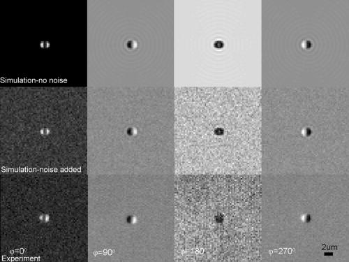

The PS-DIC image contains no amplitude information. Amplitude of weakly absorbing phase objects can be extracted separately using the same four DIC images as

Eq. 6

$$4a_1{a}_2={[{(I_{90}-I_{270})}^2+{(I_0-I_{180})}^2]}^{1∕2}.$$

This is not the same amplitude as would be measured with a bright-field microscope since $a_1$ and $a_2$ are sheared a distance $2\Delta x$ apart.³³ A comparison of simulated and experimentally acquired traditional DIC, PS-DIC and phase-shifted amplitude images is shown in Fig. 3 and discussed in detail in Sec. 5.

Fig. 3

(a) Comparison of simulated (top) and experimental (bottom) DIC with phase $\text{bias}=90\mathrm{deg}$ (left), PS-DIC (middle), and phase-shifted amplitude (right) images, computed using the input images shown in Fig. 2, demonstrates that phase-shifting removes the asymmetric phase gradient response of DIC by extracting the object phase gradient from the DIC intensity. The PS-DIC also shows an improvement in the SNR as compared to the DIC image of $3\mathrm{dB}$ in the simulated case and $8\mathrm{dB}$ in the experimental case. (b) Profiles along the direction of shear through the simulated (top) and experimental (bottom) DIC, PS-DIC, and phase-shifted amplitude images shown in (a), illustrate that equal phase gradients with opposite sign will not necessarily be imaged with the same intensity in a DIC image. The reversal in sign of the PS-DIC peaks is due to a negative sign in the phase-shifting algorithm [Eq. 4]. The $y$ axes are labeled with uncalibrated $16\text{-}\text{bit}$ values. In the simulated profile, the positive and negative peaks in intensity are 0.2809 and $-0.3413$ from the background offset. In the experimental profile, the positive and negative peaks in intensity are $0.3\times {10}^4$ and $-0.37\times {10}^4$ from the background offset.

Previous attempts to numerically integrate linear phase gradient images of arbitrarily shaped objects from PS-DIC images to obtain linear phase information produced inadequate results. These images, integrated numerically, show directional artifacts due to the direction sensitivity of DIC imaging and also due to an unknown constant of integration.^{3, 12}

4.

Methods

For direct comparison of PS-DIC and SPI results from simulated and experimental DIC images, the sample object is³⁵ a $2\text{-}\mu \mathrm{m}$ polystyrene bead $(n=1.59)$ embedded in optical cement of refractive index $n=1.55$ (Fig. 4 ). In the simulated DIC case, the bead object is a 2-D computer-generated test object or phantom with phase between 0 and $0.9\mathrm{rad}$ and amplitude of 0.93, which is representative of experimental values of 7% absorption. This percent value was derived from the difference between the average background and object amplitudes in bright-field images of the experimental object. Since the $2\text{-}\mu \mathrm{m}$ bead size falls within the depth of field of our optical system, the simulated DIC phantom used is a $64\times 64$ computer generated 2-D projection of the 3-D phase of a polystyrene bead. In the empirical case, the bead object is one of a set of fluorescent polystyrene beads dried onto a cover slip, then covered with liquid optical cement and a glass slide. The weight of the slide forces the cement to surround the beads, before being cured with a high-power UV source. The maximum change in refractive index $\left(\Delta n\right)$ of the preparations was kept as small as possible in an attempt to realistically model phase variations likely to be seen in biological applications.

Fig. 4

Phase and magnitude of the $64\times 64$ 2-D computer-generated test object with phase between 0 and $0.9\mathrm{rad}$ and magnitude representative of 7% absorption (images are shown on the right and profiles through the centers of the images shown in the panels on the left). The 3-D phase of the experimental object, a $2\text{-}\mu \mathrm{m}$ polystyrene bead, $n=1.59$ , embedded in an optical cement, $n=1.55$ , is approximated by its 2-D projection.

We also present experimental SPI results from DIC images of fixed BPAE cells in division. These cells are fixed on a prepared slide acquired from Invitrogen Corporation—Molecular Probes (Carlsbad, California, USA) and are labeled with MitoTracker Red CMXRos, BODIPY FL phallacidin and DAPI. Section 4.1 describes our method of image simulation and the implementation of the SPI algorithm. Section 4.2 describes our method of experimental image acquisition as well as points to consider when applying SPI to empirical data.

4.1.

Image Acquisition Simulation

Simulated DIC images of the phantom bead were computed from a 2-D coherent illumination model [Eq. 3] in MATLAB using the 2-D DIC transfer function.^{6, 7} The optical properties of the simulated imaging system were chosen to match those of the experimental microscope as closely as possible, using a $20\times$ , $0.5\mathrm{NA}$ , and a $7.4\text{-}\mu \mathrm{m}$ square pixel size in the image plane (equal to $7.4∕20\mu \mathrm{m}$ in the object space). The wavelength was $0.55\mu \mathrm{m}$ . For more realistic comparison with empirical results, Gaussian distributed noise with zero mean was added to the simulated DIC images used for calculation of the SPI result. Because our images are captured with a CCD camera, which is associated with photon-counting statistics,³⁶ image intensity can be modeled by a Poisson process. In DIC imaging, the light levels are in general high and thus, a Gaussian simplification may be adequate because for high photon counts the Poisson process converges to a Gaussian one.³⁷

The level of noise added was determined by the measured SNR in the experimental DIC images at each level of bias. The SNR is $17\mathrm{dB}$ for images with phase bias $\phi =0$ , $19\mathrm{dB}$ for $\phi =\pi$ , and $28\mathrm{dB}$ for $\phi =\pi ∕2$ and $\phi =3\pi ∕2$ . Figure 2 shows simulated DIC images with and without noise of the bead phantom. Additional experimental sources of error not addressed by our simulation include subpixel alignment errors, phase errors due to imperfect polarization optics, and phase differences between the orthogonal polarizations due to the high NA.

A total of eight simulated images were used to calculate the two orthogonal simulated PS-DIC images [Eq. 5]. These two images combined in the form of a complex vector [Eq. 7] were input to the SPI algorithm. The combined image was padded to twice the original size, in the space domain, with pixel values equal to the average of the background. The background value was not generally equal to zero. Padding with a constant value, rather than zero, affects only the zero-frequency value. The image was then expanded to twice the size again by doing a mirror reflection about the $x$ and $y$ axes, before transformation with a fast Fourier transform (FFT), to further minimize image processing artifacts.⁴ The transformed image was then divided by $H(m,n)$ and inverse Fourier transformed. Any zero values in $H(m,n)$ were set to one to avoid dividing by zero. As a result, spatial frequencies $2\pi m\Delta x$ (and $2\pi n\Delta y)=2N\pi$ , where $N$ is an integer, are unaffected by the filter. The mirroring process is undone by reducing the image to its original size. SPI results from simulated DIC images are show in Figs. 5 and 6 .

Fig. 5

Comparison of simulated and experimental SPI results. In the top row are the SPI results from input, from left to right, of (a) simulated images (shown in Figs. 2 and 3) without noise, (b) simulated images with Gaussian noise added, and (c) experimental images. Horizontal profiles through these images are plotted in Fig. 6. The bottom row is the phase error between the normalized SPI result, in the corresponding image above, and the normalized simulated test object phase (Fig. 4). The maximum amount of phase error between the normalized SPI results and the normalized simulated test object is less than 20% for the simulated SPI results in agreement with results published in Ref. 4. This error increases by 10%, primarily at the edges of the object, for the normalized experimental SPI result.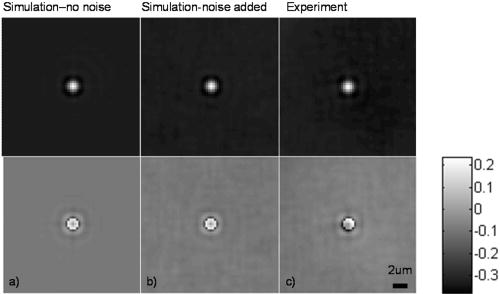

Fig. 6

Horizontal profiles through normalized SPI results, shown in Fig. 5, along with a profile through the normalized simulated test object phase. Approximately 10% of the phase error between the normalized SPI result and the normalized simulated test object phase, shown in Fig. 4, is due to a background offset.

A major limitation of this type of filtering is its sensitivity to noise. Reference 20 presents results of a method for reconstruction of optical path length (OPL) distributions based on a Weiner filter. However, this method did not produce a linear phase image because it was based on traditional, non-linear, DIC images and only one DIC image, i.e., one direction of shear.

4.2.

Image Acquisition Experimental

Empirical SPI results were produced from experimental PS-DIC images from two directions of shear. Images were captured with a Photometrics Cascade camera with $7.4\text{-}\mu \mathrm{m}$ square pixels mounted on a Zeiss Axioplan DIC upright microscope using a $20\times$ , $0.5\mathrm{NA}$ objective, and a halogen lamp source filtered with a $515\text{-}\text{to}565\text{-}\mathrm{nm}$ bandpass optical filter. Four images with phase $\text{bias}=0$ , $\pi ∕2$ , $\pi$ , and $3\pi ∕2\mathrm{rad}$ were recorded and used to calculate the two empirical PS-DIC images from each of the two shear directions. The phase bias was controlled using a Senarmont compensator rather than by laterally shifting the Nomarski prism. Figure 7 shows this configuration of the DIC microscope. The four images comprising the second shear direction were obtained using a rotating stage, which enabled the preparations to be rotated $90\mathrm{deg}$ . Two empirical PS-DIC images containing orthogonal linear phase gradient values, with amplitude information removed, were combined according to Eq. 7.

Fig. 7

Configuration of the PS-DIC microscope. A traditional DIC microscope is fitted with a rotating output analyzer and a quarter-wave plate. The Senarmont compensator configuration enables precise control of the amount of added phase shift.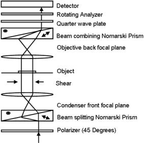

We now present a short explanation on how we use phase-correlation to align the PS-DIC images.³⁸ Traditionally, alignment through phase correlation is achieved by dividing the Fourier transform of the image to be shifted by a complex exponential whose phase angle is equal to the difference in phase angle of the shifted images in the Fourier domain. However, depending on the level of noise in the original images and the difference in image content over the shifted region, the phase shift calculated between the two images may not correspond to a single point, but encompass several pixels of the image matrix, causing errors in the alignment. Instead of using the calculated phase shift directly, we replace the calculated phase shift with a new array entirely of zeros with a single value of one in the location of the maximum of the original calculated phase shift. The Fourier transform of the new array becomes the new exponential by which the image to be shifted is divided. This ensures that all the pixels are shifted by the same amount. Note that this process shifts rows and columns but does not eliminate them. For example, if a $512\times 512$ image is shifted to the right 12 columns, columns 501 to 512 become columns 1 to 12, while columns 1 to 500, become columns 13 to 512. Once images are in register, the nonoverlapping columns must be cropped to avoid introducing error into the integration process. These images are then expanded by doing a mirror reflection about the $x$ and $y$ axes and then padded, windowed and filtered in the Fourier domain as described in Sec. 4.1.

A poor SNR in the original DIC images will degrade the SPI result. A characteristic of the spiral phase filter is that low-frequency noise is boosted more than high-frequency noise. We avoid high-frequency noise amplification by windowing the spiral phase function so that frequencies outside the system cutoff are eliminated. Additional digital signal processing artifacts can be avoided by requiring that images are not aliased by digital camera sampling.

The effects of misfocus can also degrade the SPI result and must be considered carefully especially when features of interest are on the scale of the depth of field and greater. Low frequencies from well outside the focal plane, but still present in the original PS-DIC images, only partially reconstruct the object phase outside the focal depth in the SPI result.⁵ Therefore, it is critical to be aware of the axial size of the object being studied with respect to the focal depth of the system and to adjust focus well with respect to the structure of interest. To avoid the influence of misfocus and edge effects, we crop out any out of focus objects or objects overlapping the image edge before the images are combined. The SPI result of a multilayer object must be interpreted with some previous knowledge. For example, if misfocused information is superimposed with structures of interest and cannot be cropped or if an object is embedded within a medium that is also varying with phase, it is critical to interpret the SPI result accordingly. However, this effect does not necessarily restrict the method to imaging only objects whose thickness is less than the system’s depth of field. For example, if the object of interest falls within the depth of field but is embedded within a larger medium with additional phase changes outside the depth of field, the object can be successfully imaged using this method provided the additional phase changes are far enough outside the depth of field. For thick samples, there may be some additional degradation of the resultant image (quantitative phase error) due to spherical aberration, however, misfocus, due to phase changes above and below the plane of focus, will not contribute significantly to error in the final result. Due to its natural “optical sectioning” property, the depth of field of a DIC imaging system is shorter than that of a traditional bright-field imaging system with an equivalent NA. Therefore, the axial variation of the object, in a case such as this, could be larger than would be dictated by the NA of the system. Practical examples of this case include imaging of cells grown in culture and imaging of embedded optical components in integrated optical circuitry.³⁹ Objects that are only partially in the field of view of the objective will not image linearly due to the lack of complete phase gradient information.

5.

Results

The theoretically predicted imbalance of DIC intensity along positive and negative phase gradients of a symmetric bead is demonstrated in Fig. 3. Profiles along the direction of shear through simulated and experimental DIC images with a phase bias $\phi =\pi ∕2$ show a larger difference in intensity with respect to the background offset for negative phase gradients than for positive phase gradients despite the fact that the phase of the object is symmetric. In the simulated profile, the difference in intensity between the negative peak and the background offset is 1.22 times greater than the intensity difference between the positive peak and the background offset. In the experimental profile, the difference in intensity between the negative peak and the background offset is 1.23 times greater than the intensity difference between the positive peak and the background offset. The simulated and experimental DIC images are in very good agreement confirming that this result is not due to any roughness in the experimental object. Profiles through simulated and experimental PS-DIC images show that phase shifting removes the asymmetry of the DIC phase gradient response, as well as the DIC amplitude information. The PS-DIC images show improved contrast and an improvement in the SNR of $3\mathrm{dB}$ in the simulated case and $8\mathrm{dB}$ in the experimental case. The simulated phase-shifted amplitude follows a trend similar to that of the experimental phase-shifted amplitude in that it is noisy and has poor contrast. Although the background of the simulated phase-shifted amplitude varies around the original input value, this result, as expected, is a very poor approximation of the input amplitude.

As a consequence of encoding the phase information as intensity values, direct comparison of SPI results requires calibration to a well-characterized standard because results will depend on the initial illumination parameters. The SPI results, shown in Figs. 5 and 6, are normalized to their maximum value to allow comparisons. Experimental and simulated SPI results are in agreement with results published in Ref. 4. The maximum amount of phase error between the normalized SPI results and the normalized simulated test object is less than 20% for the simulated SPI results. Reference 4 reports a maximum phase error of 17% between the normalized SPI results and the normalized simulated test object. This error increases to a maximum of approximately 30% when comparing the normalized experimental SPI result with the normalized simulated test object. Part of this error is due to a background offset of approximately 10% between the normalized SPI results and the normalized simulated test object phase. This offset is the result of convolution with a finite bandwidth filter and may be reduced by computing the filter values in the space domain.⁴⁰ As expected, there is a ripple through the background of the SPI results not present in the simulated test object phase due to diffraction at the imaging aperture not taken into account in the derivation of the SPI filter.³⁴ As a result, the maximum amount of error occurs at the edge of the object where the phase of the object is not well resolved. Normalized SPI results from simulated DIC images with and without noise differ by less than 1%, indicating that the algorithm is not sensitive to the type of noise present in the simulated images. Therefore, the increase in phase error in the experimental SPI result may be due to additional experimental sources of error not addressed by our simulation, such as subpixel alignment errors, phase errors due to imperfect polarization optics or slight misalignments of their optical axis, and phase differences between the orthogonal polarizations due to the high NA.

The potential for quantitative phase imaging of finely detailed biological structures is demonstrated with the SPI result from experimental DIC images of a partially absorptive, asymmetric object imaged with a high NA (Fig. 8 ). Figure 8 shows a fixed BPAE cell in the prophase stage of mitosis imaged at $100\times$ , and $1.3\mathrm{NA}$ , with DIC and DAPI fluorescence alongside the SPI result. The SPI result shows changes in intensity corresponding to an increased density of mitotic chromosomes visible in the fluorescence image. Phase changes that are hardly recognizable above the background in the traditional DIC image are seen with much higher contrast in the SPI result. Very little resolution of fine detail in the DIC image is lost in the SPI result. Edges of the cell and places where the cell is cropped at the edge of the image show the poorest reconstruction, which is consistent with our simulated results and those of Ref. 4.

Fig. 8

Comparison of (from left to right) a DIC image of a BPAE cell in the prophase stage of mitosis imaged with $100\times$ and $1.3\mathrm{NA}$ , an empirical SPI result from DIC images of the same cell imaged with $100\times$ and $1.3\mathrm{NA}$ , and a DAPI fluorescence image of the cell imaged with $100\times$ and $1.3\mathrm{NA}$ . An overlay of the SPI result on the DAPI fluorescence image (far right) highlights the correspondence between the two images. Arrows in the DIC and SPI images mark corresponding areas in which the SPI result exhibits increased phase contrast without loss of detail seen in the DIC image.

6.

Conclusion

Simulated DIC images of a partially absorbing phantom bead, computed using a 2-D coherent illumination model with additive zero-mean, Gaussian distributed noise, are a very good approximation to experimental images of a 3-D polystyrene beads embedded in optical cement. As predicted by this model, the intensity of traditional DIC images is not linear with the object phase gradient even at a DIC phase bias $2\varphi =\pi ∕2$ . Results from simulations and experiment confirm this for an object with a maximum phase of $0.9\mathrm{rad}$ $(\sim \pi ∕3)$ and 0.93 amplitude (7% absorption).

Phase shifting extracts phase gradient information from a set of DIC images that is linearly related to phase and is suitable for integration. The integration result is an approximation of the true phase of the object, which can be calibrated and translated into a phase measurement. Spatial frequency information normally attenuated in a single DIC image due to the particular shape of the DIC transfer function is recovered with this technique. Experimental results computed with phase shifting are consistent with results obtained from simulations.

Simulated SPI results are a good predictor of experimental SPI results. Both predict the correct shape of the input object phase. For truly quantitative SPI results, useful as a map of phase measurement, calibration of the relationship between the SPI result and the object phase must take into account both an offset and a proportionality factor. The accuracy of this method could be improved with a calibration that takes these factors into account.

Experimental SPI results of a cell in mitosis derived from DIC images taken with high NA shows the potential use of the SPI method applied to PS-DIC images for the study of density changes during the cell cycle without staining.

The need for calibration for the quantitative interpretation of results computed with the SPI method is evident. The development of such a calibration method is underway and will be presented in a future publication.