1.1.1.

Principal component analysis and linear discriminant analysis

Principal component analysis (PCA) and linear discriminant analysis (LDA) are mathematical methods that, on a statistical basis, enable data reduction and clustering into groups.⁶ There are papers on applying PCA for OCT related analysis. Weissman ⁷ used PCA for comparing the agreement of their surface recognition algorithm with the line drawn by human operators. Qi ⁸ used PCA for preprocessing. They were reducing six statistical measures for texture features to two principal components. However, using this approach they reported no benefit over using the 6-D data.

Huang and Chen⁹ also applied PCA and LDA for classification, but not on the OCT image itself. Rather, they were using a set of 25 morphological parameters to characterize ophthalmologic pathologies. These parameters were thickness and size measures that could be extracted from the OCT image. In nonophthalmic OCT imaging, such defined layers are usually not observed.

Zysk and Boppart¹⁰ reported three methods for classifying three relevant groups (adipose, cancerous, stroma) in A-scans of breast cancer biopsies. The first was taking the Fourier transform (FT) of an A-scan and using its difference from a reference (the mean of a training set) for the analysis. The second was periodicity analysis, which looks at the distance between high-intensity subsurface peaks to the surface peak. The third was a combination of both. The periodicity analysis seems to benefit from the “bubbly” structural pattern in OCT images of adipose breast tissue, which, however, is not present in every type of tissue. Part of this method, taking the FT of an A-scan, we compare with our method. (We did not implement the periodicity technique.) This enabled us to test the Fourier domain technique on sets containing more than three groups.

1.1.2.

Surface recognition

For OCT there is no established method for unsupervised surface recognition. This is, however, not straightforward as the point with the highest intensity within one A-scan is not necessarily correlated with the sample surface. This is also true for taking the first derivative of the intensity; the largest change in intensity is not necessarily at the surface. Were this the case, surface recognition could be done quickly and elegantly using a weighing of the magnitude and the derivative of the signal intensity over the single A-scan. Specifically for biological samples, this is prone to errors (cf. Fig. 1 ).

Fig. 1

(a) Denoised B-scan of a biological sample (porcine esophagus), (b) white dots mark the point of highest intensity within one A-scan (overlay over dimmed intensity image), (c) white dots mark maximum rate of change in intensity within one A-scan, and (d) surface pixels as recognised from a binary threshold mask. (b) and (c) show that the maximum intensity and derivative do not necessarily correlate with the surface.

There is a small amount of literature about surface recognition in OCT and research groups seem to have methods that seem fit for the purpose of their publication, but are not always useful to implement for a different specimen type. We found a variety of reports, e.g., shapelet-based boundary recognition;⁷ rotating kernel transformation, which emphasizes straight lines within an image;¹¹ erosion/dilation techniques on a binary threshold image;⁸ or polynomial fitting through median-blurred intensity peaks.¹²

We chose binary thresholding because it is accurate and fast. A visualization of the full process is shown in Fig. 2 .

Fig. 2

(a) Original noisy OCT image (false color log of intensity envelope data), representative for many ex vivo scans, where the sample surface, although somewhat straight, is not exactly parallel to the scanning direction; and (b) binary image using a 0.90 quantile threshold; (c) surface recognized from (b); and (d) image after wrapping.

2.1.1.

OCT device

The OCT device used in this study was a time-domain benchtop system, which was similar in design to the system described by Yang ¹³ The light source is a superluminescent diode (SLD, Superlum) with a central wavelength of $1310\mathrm{nm}$ that provided an axial resolution of $\sim 15\mathrm{\mu }\mathrm{m}$ in air and a $10\text{-}\mathrm{\mu }\mathrm{m}$ lateral resolution. The rapid delay line is realized using a double-pass mirror and a reference mirror mounted on a galvanometer (Cambridge Instruments). The data acquisition was performed using LabVIEW.

2.1.2.

Samples

As a demonstrator of proof of concept, fruit and vegetables served as readily available samples with varying structure (Fig. 3 ). Ten scans were taken of each vegetable; three vegetables of one kind form a group. In addition to this, fresh porcine specimens were obtained from a local butcher. Twenty different samples were prepared from each investigated organ, although all specimens originate from one animal. The size and shape of the samples enabled them to be placed in petri dishes for the measurements. Where necessary, samples were kept stable with needles.

Fig. 3

Representative OCT images of vegetables (after denoising, to be fed into surface recognition): (a) celery, longitudinal; (b) Celery, axial; (c) leek, longitudinal; (d) leek, axial; (e) onion; (f) potato; (g) mushroom stem; (h) mushroom top; (i) lemon; and (j) lime. All B-scans in this paper have a width of $3\mathrm{mm}$ . Note the somewhat similar appearance of (c) and (d), (g) and (h), and (i) and (j).

2.2.1.

Image

All images used in this study measure $300\times 500$ pixels, covering a 3-mm width and an approximately 5-mm depth. The log of the intensity data (time domain signal) was stored as a matrix. Values were handled in double precision format. For the automated noise reduction, a ribbon of “air,” intensity information above the surface, was regarded as background noise level.¹⁴ The mean of this plus $7\times$ the standard deviation of this background signal was used as the intensity threshold. This relatively high threshold does crudely cut off low-level signals from deeper areas. We found it, however, to be more important for our subsequent surface recognition to have a noise-free image, with the surface not being obscured by artefacts or layers.

The scanning protocol therefore required an area of air above the surface. We aimed to cover approximately 1/5 to 1/3 of the image height, as this was convenient for manual handling. The surface of the sample was positioned to ensure that the full penetration depth could be depicted on the image. Specimens were placed so that the beam angle would not cause excessive reflections. While these limitations for the distance of the probe to the sample were chosen with respect to easy handling, no measurement was taken from the same site, as that would spoil the validity of the subsequent correlation.

After thresholding, the intensity values of one B-scan were normalized to the maximum intensity peak, by scaling to the maximum peak being unity.

2.2.2.

Surface recognition and normalizing

Detecting the surface based on a binary threshold mask of the image, as shown in Fig. 2, is an approach we found to be robust for the purpose of our preprocessing. After finding no substantial influence on the result for threshold levels between 0.85 and 0.975, we arbitrarily defined a 0.95 quantile threshold for creating a binary image. The first pixel of this mask was taken as the surface. No smoothing or correction of eventual outliers (e.g., reflection artefacts) was performed. Normalizing to the surface was achieved by shifting each A-scan according to the surface vector.

Of these images, we calculated several representative measures of the depth profile of the intensity variation within one image: the mean B-scan, median B-scan, standard deviation, or the mean divided by the standard deviation¹⁵ (M/SD). Furthermore, we looked into combinations of these, e.g., M/SD and mean as two representative measures for one B-scan. We also used the FT of an A-scan to be able to roughly compare our results with the approach of Zysk and Boppart.¹⁰

3.1.1.

Surface recognition and normalizing

Vectorization reduced the processing time roughly by a factor of 4 to 5. The visual results of the unsupervised surface normalizing were effectively shown in Fig. 2d. Figure 4 shows how normalizing to the surface affects the mean and the M/SD of a B-scan.

Fig. 4

(a) Mean A-scan of original data, (b) mean A-scan of surface normalized image, and (c) M/SD along row of A-scans: (—) surface normalized and (- - -) original.

3.1.2.

Vegetables—separate A-scans

In a first approach, we used 10 images of three vegetables, resulting in 30 images or 9000 A-scans. Performing PCA on the surface normalized A-scans [Fig. 5A ] or nonsurface normalized FT curves [Fig. 5B] show a tendency to group, but also considerable overlap. Note that the plots in Fig. 5 show only the two most significant (ANOVA) PCs for classification against each other. The subsequent LDA separates on the basis of a pool of several PCs (25 in the examples of this paper).

Fig. 5

PCA of three vegetables, 10 images each. The plots show the PCs of 9000 A-scans with the two highest scores (determined by ANOVA) out of 25: (a) surface normalized and (b) FT of A-scans (no surface normalization). Legend: 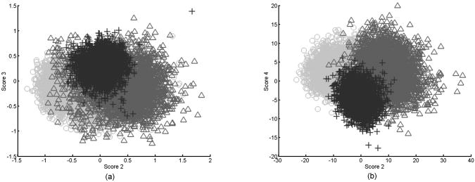$\circ =\mathrm{celery}$ ; $△=\mathrm{onion}$ ; $+=\mathrm{mushroom}$ .

Table 1 shows the performance of classification models for this case. For the amplitude of the frequency content, surface normalization does not improve the classification. For classifying time domain data (spatial information), surface normalization yields a higher rate.

Table 1

Comparison for classification of three A-scan representations: the FT, the amplitude of the FT, and time domain data.

3.1.3.

Data reduction prior to PCA

The classification rates in Table 1 are not disappointing, but take a long time to calculate. Hence we reduced the B-scan to a representative measure, as shown in Fig. 6 . From the mean of these images, the separation is clearer than in Fig. 5. For this approach, surface normalization has a stronger impact than before: classification was correct in 93.3% for the surface-normalized data [Fig. 6A], but only 33.3% for not-surface-normalized data [Fig. 6B].

Fig. 6

PCA of three vegetables, 10 images each. The data points show the two highest scoring PCs (ANOVA) of the 30 representative measures: (a) surface normalized and (b) no surface normalisation. $\circ =\mathrm{celery}$ ; $△=\mathrm{onion}$ ; $+=\mathrm{mushroom}$ .

3.1.4.

Data reduction—large dataset

A large data set consisting of 330 images, categorized into nine groups, was used to assess various representative measures. These 99,000 A-scans could not be fed into analysis on a Pentium type processor with $1\mathrm{Gbyte}$ of RAM, so it was essential to extract a representative measure. Table 2 shows the results for data reduction. For time domain data, models created using the mean normalized by the standard deviation (M/SD) had the best results, as shown in Table 2. For models from the FT of an A-scan, the standard deviation (SD) has the highest classification score. After LOGO cross-validation, the model constructed from the mean values has a higher score.

Table 2

Training performance (TP) and cross-validation (CV) of a data set consisting of nine groups; seven groups of 30 images each and two groups of 60 images each (330 representative measures).

3.2.1.

Vegetables

A different set consisting of 330 images, categorized into seven groups, was classified correctly (after LOGO cross-validation) as follows: SN-MSD, 91.8%; AFT-M, 93.9%; and AFT-SD, 79.1%. For comparison, the non-surface-normalized approach reached 32.0% in this case.

3.2.2.

Similar image types

In the next step, we assessed the classification of similar images, i.e., measurements of one type of vegetable with different orientation, or similar images (lemon versus lime). Representative B-scans are shown in Figs. 3G, 3H, 3I, 3J. Classification results for 30 images each are shown in Table 3 .

Table 3

Classification rates after LOGO cross-validation; training models were created for pairs of similar images ( 2×30 images for a pair).

3.2.3.

Similar images in a large group

If groups are similar, further added groups do decrease the power of the separation. To show this, we grouped two vegetables to yield four groups. Separation is affected when these two groups must be distinguished not only from each other, but also among other data, as shown in Table 4 .

Table 4

Classification rates after LOGO cross-validation; training models were created for sets of pairs of similar images ( 2×30 images for a pair).

3.2.4.

Preliminary tissue pilot study

Extending on the vegetable findings, we used porcine samples for a preliminary tissue pilot study. We measured 20 sites each of four different tissue types (tongue, esophagus, tracheae, and bronchioles). Representative images are shown in Fig. 7 . The results for PC-fed LDA classification are encouraging. After LOGO cross-validation, the four, albeit clearly distinct tissue types, are classified 90.0% (SN-MSD), 82.5% (AFT-M), and 70.0% (AFT-SD) correctly.

Fig. 7

Representative OCT images of porcine samples: (a) squamous lining of the esophagus, (b) tongue, (c) tracheae, and (d) bronchioles. Each image covers $3\mathrm{mm}$ in width.

To see whether more subtle changes can be picked up, we looked at samples from one tissue type (esophageal) measuring them in a fresh state, after degradation for 5 days, and after application of 5% acetic acid, a contrast agent that is used in clinical settings. These three groups can be separated well between each other in 91.7% (SN-M/SD), 93.3% (AFT-M), and 76.7% (AFT-SD) of the cases (LOGO cross-validated).

4.1.1.

Time domain data and frequency content

Classification requires preprocessing. Both methods, the amplitude of the FT of an A-scan and the surface normalized A-scan, give good results. The FT we used to create a model differed in four points from that of Zysk and Boppart.¹⁰ First, our denoising and normalizing, as already described, was different. Second, we were using the FT of the A-scan for classification, and not the difference from a reference. Third, Zysk and Boppart report that they did perform surface normalizing (“truncating”) prior to FT, whereas we found that to be beneficial only when feeding the real and the imaginary part of the FT. However, we achieved better results when using the amplitude of the FT directly of the non-surface-normalized A-scan. Finally, we took a representative measure for a set of A-scans and classified the set, rather than classifying single A-scans.

It then probably depends on the sample structure, e.g., the presence of distinctive periodic patterns, whether the frequency information or time domain data enable a better classification. Time domain data must be surface normalized. This requires a robust and quick surface recognition and means an additional computational step.

We are aware that the data for this paper are suitable for binary thresholding as surface recognition, and that the converse is not necessarily always the case. Such scenarios could be imagined where the surface of interest is covered by a layer of mucus, a sheath, a balloon, or something similar. Research into more robust and reliable surface detection algorithms would therefore be beneficial.

4.1.2.

Representative measure

Reducing the data to a representative A-scan is necessary; our Pentium type processor with $1\mathrm{Gbyte}$ of memory was not able to handle data sets of tens of thousands of A-scans. More powerful computers are of course available, but it is conceivable that OCT data will stretch these resources to the limit for the near future. We found that the M/SD of a surface-normalized B-scan or the mean of the frequency content yield good results. For instance, at separating two similar celery orientations, the SN-MSD approach practically fails (56.7%), whereas the AFT-SD reaches over 80%. For classifying porcine tissue, the SN-MSD approach had the best result. In the case of variations within a B-scan, such as in Fig. 8 , standardizing using the SD does improve results for the subsequent classification.

Fig. 8

(a) Surface-normalized B-scans, where the depth profile is homogeneous across the scan width and can be well described by a mean A-scan, and (b) structures that result in different A-scans, e.g., A-scans at the two white lines will be different. In this situation, a standardized mean seems to better represent the B-scan.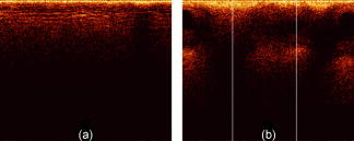

In terms of preprocessing, we also investigated mean centering, and using more than one representative measure (data not shown). We did not perform any correction of the surface vector in this study, although that is beneficial (data not shown). Further, the performance of LDA can be improved by feeding an optimum number of PCs. However, this optimum depends on the number and kind of groups in the classification model. The different sample groups in this study do have different optimum numbers of PCs. For instance, for classifying four tissue types, the classification performance, using 25 PCs, was 90.0% (SN-MSD) and 82.5% (AFT-M). For these groups, the optimum for SN-MSD would be reached by feeding 11 PCs (97.5% LOGO cross-validated), and for AFT-M 7 PCs (91.3%). For the purpose of this demonstration, we decided to keep a fixed number of PCs. It might well be worth investigating a combination of two or more measures, and automatically refining extracted measures. However, this is beyond the scope of this paper and is probably only worthwhile when refining the technique for a dedicated purpose. Summarizing, it is possible to improve results by fine-tuning and combining parameters.

4.1.3.

Speed

One criterion for processing is speed. OCT acquires data in real time and hence the subsequent analysis should not impact on this characteristic. Preprocessing does slightly delay results: on a 2.80-GHz Pentium 4, classification of 330 B-scans takes approximately $85\mathrm{s}$ , of which $73\mathrm{s}$ are required for surface normalization and extracting a representative measure. That corresponds to roughly 60,000 A-scans/min and makes us confident that the claim of providing a near real-time modality remains justified. It would be quite remarkable for a human operator to classify 330 images in $1\frac{1}{2}\min$ . However, we were only using a run-length-encoded programming language for proof of principle; compiled programs run much faster.

4.2.1.

Relevance for medical data

The fact that the algorithm reaches over 90% accuracy in certain cases is reassuring when looking at obviously different images, but for our data set the displayed approach is also able to differentiate images reasonably well that are difficult to tell apart by the eye. Further, the algorithm is still able to classify similar images among a pool of other structural data.

This is important as we plan to apply this algorithm to medical data. There, we expect a larger variation among healthy individuals, and only eventually the small, but significant alterations for early, nonsymptomatic disease. As an example, we note epithelial cancers, carcinomas, where the epithelial thickness of the healthy population can vary considerably due to various factors. However, the subtle alterations of proliferative epithelial cells close to the basal layer are probably the feature that can be picked up by OCT scans. It still remains to be assessed whether the algorithm would fail in such scenarios.

4.2.2.

Limitations and benefit

In this study the imaging protocol is strict in the sense that it requires the penetration depth to be fully exploited and to leave an area of air above the surface. However, most imaging must adhere to a protocol. As long as the operator is made aware of the requirements, we believe this limitation not to be substantial. After all, we have acquired thousands of images in this way.

The advantage we see in the presented algorithm is that the few parameters utilized here are robust enough for the analysis to be automated and in near real-time. It does not require assigning areas of interest. It does not rely on specific structures such as previously reported methods, but can still be used in combination with these algorithms. Hence, this algorithm is straightforward to implement for existing OCT data.

Note that, although we were taking representative measures of B-scans, this approach will work on volumetric data. For example, taking a representative measure of a volume consisting of $20\times 20$ A-scans on a system with $10\text{-}\mathrm{\mu }\mathrm{m}$ lateral resolution will enable classification of $25\text{“}\mathrm{tiles}\text{”}∕{\mathrm{mm}}^2$ , which is still superb for targeting clinical treatment.

4.2.3.

Further work

Previous studies^{16, 17} have shown that expert histopathologists do not always fully agree on classification of tissue specimens, and an algorithm with lower than 100% correct classification can still outperform subjective human assessment. In clinical work, OCT data would have to be compared to histopathologic results. Even though there are significant discrepancies found between expert pathologists on particular pathology groups,^{16, 17} histopathology is defined as the gold standard. Therefore, we must base our analysis on the assumption that the sample pathology defined by histopathology is correct. In this study, we did not investigate the performance of the algorithm against a human operator, and hence assumed a 100% correct classification as a reference baseline. In the future, we intend to compare classification results with those achieved by histopathologists on the same OCT images from biological specimens.

The next step is testing this algorithm on medical OCT images. We expect it to distinguish structurally different pathologies correctly. In ongoing work, we are investigating how well it classifies disease groups with quite similar appearance, such as mild and moderate dysplasia in early cancer development.