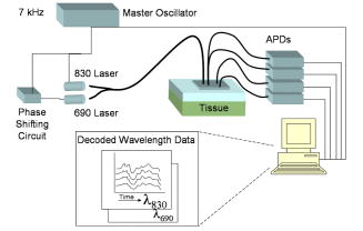
1.

Introduction

Near-infrared spectroscopy (NIRS) has been used since the 1970’s¹ to monitor cerebral blood volume and oxygenation noninvasively. Light in this wavelength regime can diffuse far enough (several centimeters) to penetrate through the scalp and skull, explore the outer regions of the cerebral cortex, and return to the surface for collection. Recordings of diffuse reflectance at two or more wavelengths permit calculation of oxy- and deoxyhemoglobin concentrations ( $\left[{\mathrm{HbO}}_2\right]$ and [Hb]), based on the distinctive absorption spectra of the two hemoglobin states.

In cerebral stimulation studies, the key parameters are often the temporal changes in $\left[{\mathrm{HbO}}_2\right]$ and [Hb] rather than their absolute levels. Measurements of continuous-wave (cw) diffuse reflectance hence can provide insight into the functional activity of the brain noninvasively, under the assumption that scattering properties of the head do not vary in time. A single-source-location, single-detector “optode” provides a running measurement of volume-averaged hemodynamic changes. NIRS studies have used such optodes to monitor responses to stimuli at specific locations,^{2, 3, 4} as well as grids of many such optodes for topographic, functional NIRS imaging. ^{5, 6, 7, 8}

From the average human subject, single-event NIRS activations cannot routinely be observed above baseline levels of hemodynamic activity. To resolve significant activation responses, most studies average over multiple stimulations per subject and often over multiple subjects as well. The signal averaging reduces interference from uncorrelated hemodynamic activity in the cortex and in the overlying scalp. Any experimental refinements that reduce the burden of signal averaging should increase the speed and per-subject success rate of NIRS.

The most straightforward refinement is to employ additional detectors closer to or farther from the source, thereby monitoring overlapping volumes. A weighted subtraction of the readings eliminates some of the hemodynamic interference. Typically, this correction has involved fixed parameters based on additional information (e.g., anatomical priors from MRI⁹); assumptions about baseline optical properties, layer thicknesses, and photon path distributions^{10, 11}; model-based multivariate calibration techniques¹²; or full 3-D tomographic reconstructions.^{13, 14, 15}

A recently proposed alternative is to base the correction directly on the shape of the time series recorded at two detectors, with the additional detector placed close to the source.^{16, 17} In this approach, the “near” detector (5 to $15\mathrm{mm}$ from the source) probes the scalp nearly exclusively. This detector’s recording is treated as physiological “noise” and removed, in some fashion, from the larger-distance $(\sim 30\mathrm{mm})$ recording, with the intent of enhancing signals pertinent to the brain. Particular methods of noise removal that have been explored in simulation include weighted subtraction¹⁶ and higher-order adaptive filtering.¹⁷ In both studies, the noise removal uncovered stimulus responses that had been masked by hemodynamic noise in the scalp and brain.

This approach is distinct from other two-detector paradigms,^{18, 19} in which measurements are made at two “far” detectors (e.g., at 30 and $40\mathrm{mm}$ from the source), each of which samples the cortex substantially. The subtraction of time series is designed, in those cases, to eradicate the contribution from the scalp layer, as if the probe were placed directly on an exposed cortex. This is desirable for instruments designed to monitor absolute cerebral oxygenation. For functional NIRS, however, it is more relevant to emphasize trends that are unique to the cortex. Systemic arousals present in both layers, which would be preserved by this sort of subtraction, are not of primary interest.

The simulation studies referenced here modeled the hemodynamics of the scalp and brain as homogeneous, layer-wide fluctuations. Indeed, this or some equivalently simple model must be invoked when only two detectors are involved. Homogeneous-layer models have been used widely in the interpretation and processing of NIRS signals. ^{11, 20, 21, 22}

In practice, however, the scalp and cortex exhibit some hemodynamic heterogeneity, limiting the validity of such models. For any two-distance filtering method to be useful, this heterogeneity cannot be too great. While the hemodynamic variations need not be completely layer-like, they need to contain a substantial layer-like component to ensure that the separated detectors respond to correlated noise trends. To our knowledge, the validity of using homogeneous-layer models for NIRS measurements has not been directly studied experimentally.

In this work, a fundamental examination of the heterogeneity of optical fluctuations in the head, and the corresponding influence on NIRS signals, was performed. Geometries with various source-detector arrangements were designed to test whether hemodynamic changes in the human head exhibit a component of layer-like behavior on the scale of a few centimeters. Because the large heterogeneity in static optical properties of typical heads, the variability between subject heads, and the variability between subject hemodynamic responses have not been extensively characterized and are hard to model with experimental phantoms or computer simulations, recordings from human volunteers were emphasized at this stage, despite the inherent complexity.

Targeted stimulations (e.g., finger tapping or pattern watching) were not used in the fundamental tests because of the inability to standardize the location of focal responses. Instead, baseline hemodynamic fluctuations were measured over the prefrontal cortex of subjects at rest. Baseline fluctuations are always present as biological noise, even in stimulation studies.²³ Contributions of physiological processes to background noise in various NIRS frequency regimes have been characterized,^{24, 25} and efforts have been made to reduce these signals through combinations of modeling, adaptive filtering using auxiliary measurements, and basis function deconvolution techniques.²⁶ In the studies here, the baseline fluctuations simply provided a noise level that we wished to reduce via the two-detector approach, without any physiological interpretations. Following these fundamental tests, studies of two simple stimulation protocols were also conducted to compare two-detector and traditional single-detector NIRS recordings.

2.

Methods

2.1.

Overview

Volunteers’ heads were first tested for layer-like hemodynamic behavior using the measurement geometries summarized by Figs. 1a and 1b . In both cases, there was a single source $S$ , a main detector $A$ $33\mathrm{mm}$ away, and three extra detectors ( $B$ , $C$ , and $D$ ). In Fig. 1a, the extra detectors were positioned along the arc of a circle, $r=33\mathrm{mm}$ , centered at $S$ (henceforth “circular geometry”). In Fig. 1b, they were placed along the line segment connecting $A$ to $S$ (“linear geometry”). Figure 1c shows a hybrid of the circular and linear geometries that was used in subsequent studies.

Fig. 1

Configuration geometries used for source fibers and detector fiber bundles. All cases feature a source location $S$ and a main detector $A$ $33\mathrm{mm}$ away. The (a) circular and (b) linear geometries differ in the placement of the three other detectors and in the corresponding photon exploration volumes. (c) Geometry provides simultaneous circular and linear displacements from detector $A$ with the same detector-detector spacing of $28\mathrm{mm}$ .

Linear and circular geometries were employed because they probe underlying tissue differently. Consider monitoring a system of two homogeneous layers experiencing different hemodynamic trends. In the linear geometry, the time series recorded by detectors $B$ , $C$ , and $D$ would be increasingly dissimilar from $A$ ’s due to changes in how the two layers are sampled [note differences in the depths of the sketched photon exploration volumes in Fig. 1b]. This increase can be quantified by the root mean squared (rms) amplitude of a residual time series, discussed later. In the circular geometry, where the photons explore equally deeply, the difference would not increase because the relative samplings of layers are identical. This greater difference in the linear geometry is the signature of what we call “layer-like” hemodynamic changes in the human head.

2.2.

Instrumentation

A cw NIRS system was constructed using laser diodes emitting at 830 and $690\mathrm{nm}$ . The layout is illustrated in Fig. 2 . To reject contributions from ambient light, both diodes were amplitude modulated at the same frequency of approximately $7\mathrm{kHz}$ , with the $690\text{-}\mathrm{nm}$ diode phase delayed by $90\mathrm{deg}$ to permit digital in-phase and quadrature (IQ) lock-in detection. Each laser delivered approximately $1.5\mathrm{mW}$ of power to the head via a custom-built fiber optic probe. Four avalanche photodiodes (APDs) (Hamamatsu C5460-01) simultaneously detected light from detection fiber bundles at different spatial locations relative to the source delivery fiber bundle, producing time series of changes in optical density $[-\log I(t)∕I_0=\mathrm{\Delta }OD(t\left)\right]$ . The output data rate from the digital IQ lock-in routine was $20\mathrm{Hz}$ . The signal-to-noise ratio of the APD voltage outputs ranged from 60 to 25, depending on the particular optical properties of individual subjects. Since these studies required calculation of differences between time series, care was taken to maintain approximately equivalent signal-to-noise ratios along all detection channels for a given subject, to ensure that signal differences pertained to physiological fluctuations and not instrument noise.

Fig. 2

System layout for single source, multidetector cw NIRS system.

Each comparison between two time series was characterized by the choice of geometry and by the detector-detector separation $\delta$ . The circular geometry provided $\delta$ values of 5, 6, 11, 23, 28, and $33\mathrm{mm}$ using all combinations of detectors. The linear geometry provided $\delta$ values of 12, 20, and $28\mathrm{mm}$ from the farthest detector $A$ . All subtractions involved at least one source-detector separation $\rho$ of $33\mathrm{mm}$ , since that distance is typical of single-detector NIRS studies and it is the nonuniquely cerebral signals in such measurements that we aim to reduce.

2.3.

Data Processing

The instrumental time series $\mathrm{\Delta }OD\left(t\right)$ from each detector was low-pass filtered by subtracting a moving boxcar average with a window of $20\mathrm{s}$ , and high-pass filtered by a first-order Savitsky-Golay filter with a window size of $1.5\mathrm{s}$ . These filters approximately provide a bandpass of 0.05 to $0.67\mathrm{Hz}$ , heavily dampening heartbeat pulsations, and removing very low frequency oscillations.²⁴

The dissimilarity between various time series was quantified using an rms metric. One signal was scaled to fit the other in a least-squares (LS) sense, as motivated by previous theoretical and Monte Carlo studies.¹⁶ Representing the two time series measurements by vectors $\mathbf{F}$ and $\mathbf{N}$ , the resulting residual was $\mathbf{R}=\mathbf{F}-\alpha \mathbf{N}$ , with $\alpha \equiv (\mathbf{F}\cdot \mathbf{N})∕(\mathbf{N}\cdot \mathbf{N})$ being the scaling coefficient that minimizes the root mean square of $\mathbf{R}$ . For short, we call $\mathbf{R}$ the “corrected NIRS” or “C-NIRS” signal. $\mathbf{R}$ reports the hemodynamic trends in $\mathbf{F}$ that are mathematically uncorrelated (orthogonal in time) to those present in $\mathbf{N}$ . In the case where $\mathbf{N}$ corresponds to a near, “scalp-only” measurement at $5\mathrm{mm}$ , trend $\mathbf{R}$ is uncorrelated with the scalp hemodynamics. As noted in the Introduction in Sec. 1, higher-order adaptive filtering or other methods could also be used to generate a conceptually similar C-NIRS residual. LS fitting is essentially the same as creating a first-order adaptive filter over the entire time window and using the scale factor for all time points. The LS approach provides a suitable dissimilarity metric with a minimum of free parameters.

Figure 3 illustrates the least-squares processing steps using representative data at $830\mathrm{nm}$ from one subject. In the linear geometry, the nearer-distance ( $B$ , $C$ , and $D$ ) time series (Fig. 3, upper left) were scaled to fit $A$ . The rms amplitude of the resulting residual (Fig. 3, upper center) was then computed as a scalar measure of difference between the two signals (Fig. 3, right). For the circular probe case (Fig. 3, lower plots), every possible combination of two detectors was used to calculate residuals as a function of $\delta$ .

Fig. 3

Calculation of the rms metric for differences between NIRS time series. Left column: simultaneous NIRS time series (units of $\mathrm{\Delta }OD$ , 830-nm channel) from the four detectors $A$ through $D$ recorded in linear (top) and circular (bottom) geometry. Middle column: residual time series created by least-squares fits of one time series to another, as described in the text. The $\delta$ value gives the detector-detector separation. Right column: rms amplitudes of each residual time series, plotted versus $\delta$ . Blue crosses: linear geometry; black circles, circular. The amplitude increases more rapidly for the linear geometry, as predicted by a homogeneous two-layer hemodynamic model. (Color online only.)

The goal of the initial studies was to study layer-like optical fluctuations, not to extract hemoglobin concentrations. In these cases, C-NIRS residuals from the $\mathrm{\Delta }OD$ time series were analyzed directly. No assumptions about layer thicknesses or photon pathlengths were required to create the residuals, as the scaling factors were provided adaptively by the least-squares fits.

In later studies, particularly those related to stimulations, the main interest was in hemodynamic parameters. This required both a C-NIRS filtering step and an OD-to-concentration conversion. Since both steps are linear, in an ideal system the operations would commute. In practice, uncertainty about the relative pathlengths traveled by 690- and 830-nm light from source to detector causes cross talk between the oxy– and deoxyhemoglobin calculations. As such, results differ depending on whether the filtering is performed in OD or concentration mode. While the two methods produced qualitatively similar results, for reporting purposes, we chose the concentration mode to permit filters for oxy- and deoxyhemoglobin to optimize separately.¹⁷ As such, first the near and far $\mathrm{\Delta }OD$ series were converted to near and far hemoglobin $\mathrm{\Delta }c$ series, and then C-NIRS residuals were created for each hemoglobin species. We found that assuming equal pathlengths at the two wavelengths kept the cross talk at an acceptable level for all channels, as judged by the observation of strong heartbeat signals (prior to bandpass filtering) for calculated oxyhemoglobin and only faint ones for deoxyhemoglobin.

Although the shape of a hemoglobin concentration trend is generally more important in NIRS than its amplitude, the values were converted to approximate molarity by assuming a pathlength factor of 5 at the far channel, derived from Monte Carlo simulations.¹⁶ No assumption about pathlength at the near channel was necessary, again because of the adaptive nature of the least-squares scaling.

2.4.

Subject Measurement Protocols

2.4.1.

Baseline hemodynamics, four locations

A first, exploratory protocol looked for evidence of layer-like hemodynamics using the linear and circular geometries of Figs. 1a and 1b. The collection fibers were devoted all to one geometry and then all to the other, to study as many detector-detector separations $\delta$ as possible and choose one that most emphasized layer-like effects. Swapping between the two geometries took less than five minutes.

Adult subjects in this and all subsequent studies were consented under protocols approved by the University of Rochester Research Subjects Review Board (number 12258). In this first study, 21 subjects were seated and asked to remain quiet and motionless during data acquisition. Since the goal was to study the spatial variability of hemodynamic signatures under baseline conditions, subjects were not presented with any stimulation or mental challenge. First, the circular probe was placed over the left prefrontal cortex, and two separate one-minute measurements were acquired. The probe was then shifted a few centimeters to the subject’s left and two more measurements were acquired. The motivation behind selecting the forehead was to avoid interference from hair. After the four circular probe measurements, the delivery and collection fibers were inserted into the linear probe and two one-minute measurements were taken over approximately the same two locations the circular probe was placed. Exact coregistration was not essential for the study. For each data run, rms values were calculated at various values of $\delta$ , via the process illustrated by Fig. 3.

2.4.2.

Baseline hemodynamics, two locations

In a subsequent study of nine subjects, the probe was reconfigured into the combined geometry of Fig. 1c, with the additional detector locations now displaced from $A$ both linearly $\left(B\right)$ and circularly $\left(D\right)$ with the same value of $\delta =28\mathrm{mm}$ . As before, subjects sat quietly with the probe over the left prefrontal cortex for one-minute measurements. In this study, rms values from linear and circular geometries could be directly compared from the same run, because the $A$ recording was common to both. This permitted more quantitative analysis of the layer-like behavior, at the expense of doing so at only one value of $\delta$ . Calculations were also performed using $C$ rather than $B$ as the near detector and $D$ as the main far detector. Three one-minute data acquisitions were taken from each subject, resulting in a total of six measurements per subject.

2.4.3.

Stimulations

Two event-related stimulation protocols were also explored: a systemic stimulation that is not specific to the brain (the Valsalva maneuver), and a visual stimulation that has been shown to elicit localized responses in the visual cortex (a flashing checkerboard pattern).^{15, 27} The goal in both cases was to compare single-channel and C-NIRS time series.

Valsalva maneuver

The Valsalva maneuver consists of a sustained, forced expiratory effort against a closed airway. The strong hemodynamic response produced by the Valsalva maneuver is not specific to functional activity in the brain, but rather is systemic. Typically, this response is characterized by a large increase in $\left[{\mathrm{HbO}}_2\right]$ and a smaller increase in [Hb]. In the protocol, the subject was seated with the probe placed over the left side of the forehead just below the hairline. The Valsalva maneuver was executed three times for a duration of $10\mathrm{s}$ between rest intervals, which varied randomly from 12 to $18\mathrm{s}$ . The total acquisition time was $90\mathrm{s}$ .

Visual contrast

Visual stimulation was provided by a flickering radial checkerboard pattern, as shown in Fig. 4 . The pattern was presented filling a $15\text{-}\mathrm{in.}$ laptop screen, approximately 18 to $24\mathrm{in.}$ from the seated subject. During stimulus periods, the contrast of the pattern would reverse at a rate of $10\mathrm{Hz}$ . During rest periods, the subject was shown a solid gray screen with a small cross-hair in the center to maintain a central fixation point. Stimulations were for $10\mathrm{s}$ , preceded by 15-s rest periods. The entire measurement lasted $3\min$ .

Fig. 4

Checkerboard pattern used in the visual stimulation study.

The probe, in the configuration shown in Fig. 1c, was placed over the occipital lobe. Using the inion as a fiducial marker on the scalp, the probe was placed approximately 1 to $2\mathrm{cm}$ above the inion in a central location. Since the accuracy of this placement method was not ideal²⁸ and the probe covered only a $2\times 3\text{-}\mathrm{cm}$ area of the head, several measurements were taken, randomly sampling multiple locations within $3\mathrm{cm}$ of the estimated central location of the visual cortex. Two subjects were studied, with a total of three and six probe positionings, respectively. For each subject, all runs were combined into a block average.

3.

Results

3.1.

Baseline Hemodynamics, Multiple Locations

Figure 5 shows resting rms values of $\mathrm{\Delta }OD$ residuals from four representative subjects at both interrogation wavelengths as a function of $\delta$ . Each data point represents the average rms value from the four measurements taken at the two adjacent prefrontal locations. Given that the values being averaged are rms least-squares residuals from four separate one-minute time series of hemodynamic noise, the percent variations are surprisingly small. While magnitudes varied across subjects, the rms values consistently increased as a function of $\delta$ for the two probe configurations (19 out of 21 subjects), with noticeably larger values for the linear configuration, particularly at larger $\delta$ separation values. The results provide strong indications of the presence of layer-distinct hemodynamic trends within the volume probed.

Fig. 5

rms signal difference $\left(\mathrm{\Delta }OD\right)$ as a function of relative detector separation $\delta$ , measured on four individual subjects at $830\mathrm{nm}$ (above) and $690\mathrm{nm}$ (below). Blue crosses: linear geometry; black circles, circular. (Color online only.)

3.2.

Baseline Hemodynamics, Two Locations

The subsequent study using the combination geometry provided rms time series differences for $\delta =28\mathrm{mm}$ in both geometries simultaneously. Consistent with the trend observed in the previous study, the linear geometry routinely produced larger rms values. For the $i$ ’th subject (six measurements), the fractional increase $FI$ in the rms difference was calculated as

Eq. 1

$${\mathrm{FI}}_i=⟨\frac{{\mathrm{rms}}_{\mathrm{lin}}-{\mathrm{rms}}_{\mathrm{circ}}}{{\mathrm{rms}}_{\mathrm{circ}}}⟩i,$$

where the brackets indicate an average over six measurements.

Figure 6 displays $FI$ for the nine subjects. In this case, to emphasize physiological meaning, the C-NIRS step was performed in concentration mode, as discussed earlier. Positive values, which at both wavelengths occur for eight of the nine subjects, indicate additional signal difference present in the linear measurements relative to the circular ones. The mean $FI$ value is significantly greater than 0 for concentration changes in both species of hemoglobin, as determined by $t$ -test $(p_{{\mathrm{HbO}}_2}=5.5\times {10}^{-10},p_{\mathrm{Hb}}=2.8\times {10}^{-8})$ .

Fig. 6

Fractional increase $FI$ in rms signal difference at $\delta =28\mathrm{mm}$ when the arrangement of detectors is linear rather than circular, measured for nine subjects. The two geometries were explored simultaneously using the combination geometry of Fig. 1. $FI$ values were calculated in units of concentration for both (a) oxy- and (b) deoxyhemoglobin.

This study also permitted an estimate of the scalp-layer trend’s contribution to the overall signal detected at $\rho =33\mathrm{mm}$ . The percentage decrease in rms amplitude was calculated between the entire (unsubtracted) $A$ signal $\left(33\mathrm{mm}\right)$ in the linear probe configuration and the residual of $A$ fit by $D$ (linear geometry, $\rho =5\mathrm{mm}$ ). The fraction of signal removed can then be estimated by computing $(rm{s}_{\mathrm{NIRS}}-rm{s}_{\mathrm{CNIRS}})∕rm{s}_{\mathrm{NIRS}}$ . Across the subject population, an average of $60\pm 25\%$ of the signal fluctuation was removed.

3.3.

Stimulation Protocols

3.3.1.

Valsalva maneuver

Figure 7 shows a typical measured response to the Valsalva maneuver. Displayed are both the full time course and the block average of the three cycles. The protocol produced clear and reproducible responses to each stimulus. As expected, there is a strong increase in oxygenated hemoglobin concentration during the maneuver, followed by an overshooting negative concentration change. The scaled 5-mm signal closely mimics the 33-mm signal for each hemoglobin species. As a result, the C-NIRS $\left[{\mathrm{HbO}}_2\right]$ residual is featureless compared to the single-detector signals, and the magnitude of residual hemodynamics is consistent with that found in resting subjects. Comparing rms amplitudes of NIRS and C-NIRS signals across the entire subject pool of seven volunteers, on average $63\pm 13\%$ of the $\left[{\mathrm{HbO}}_2\right]$ signal measured at $33\mathrm{mm}$ was characterized as not uniquely cerebral in origin and removed.

Fig. 7

Representative time series and block averages of three Valsalva events from one subject, in units of $\Delta \left[{\mathrm{HbO}}_2\right]$ and $\Delta$ [Hb]. Above: single-detector NIRS recordings at $33\mathrm{mm}$ (solid lines) and $5\mathrm{mm}$ (dashed lines). The 5-mm recordings have been scaled by least squares to fit the 33-mm data, as described in the text. Stimulus intervals are indicated by shaded regions. The plot on the right shows the block average, with a strong oxyhemoglobin response. Below: C-NIRS residual signals for both hemoglobin species. The oxyhemoglobin activations have been removed, indicating that the activation was not unique to the cortex.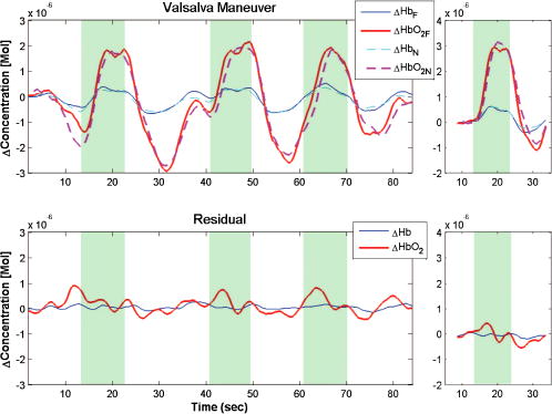

3.3.2.

Visual stimulation

Figure 8 shows representative data from the two subjects who underwent the visual stimulation protocol. Here the near measurement (scaled via least squares) is overlaid on top of the far measurement. Once again, the large fluctuations present in the far measurement are closely tracked by the near measurement. Across all the measurements of both subjects, an average of $50\pm 15\%$ of the original NIRS-derived $\left[{\mathrm{HbO}}_2\right]$ amplitude was removed. Block averages across all stimulus periods (36 and 72 stimuli for the two subjects) processed by both standard and corrected NIRS approaches are shown in Fig. 9 . C-NIRS signals show the anticipated increase in $\left[{\mathrm{HbO}}_2\right]$ responses aligned with the stimulation onset, while the single-detector NIRS plots are dominated by large fluctuations on top of the activations with no obvious interpretation.

Fig. 8

Representative time series of $\Delta \left[{\mathrm{HbO}}_2\right]$ and $\Delta$ [Hb], at 33- and 5-mm source-detector separation, from the visual stimulus protocol. Hemoglobin changes at $5\mathrm{mm}$ (scaled by least squares) again track the 33-mm recordings closely. Shaded regions indicate periods of checkerboard flashing.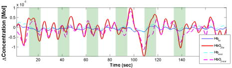

Fig. 9

Block averages of single-detector NIRS and two-detector C-NIRS responses from each of the two subjects in the visual stimulation protocol. All trials, at multiple probe positions, were included. Both C-NIRS averages exhibit straightforward stimulus-correlated responses, while the NIRS recordings have multiple features without obvious interpretation.

4.

Discussion

The best examples of NIRS recordings in the literature demonstrate that the method can detect localized, cerebrally specific, event-related hemodynamic activity during a variety of stimulation protocols. The promise of such results is tempered by the difficulty of obtaining similar quality signals from the majority of subjects. For most subjects, baseline levels of hemodynamic activity are usually larger than or comparable to event-related responses. For this reason, signal-isolation techniques such as signal averaging or volumetric discrimination must be applied.

This work tested the foundations for a two-detector approach intended to reduce hemodynamic background via depth-localized measurement. While the technique does not involve the complexity of 3-D tomographic analysis, it can isolate hemodynamic trends that are unique to the brain (i.e., uncorrelated with trends in the scalp) using minimal a priori assumptions. Significantly, it performs the subtraction without requiring estimates of local scalp and skull thickness and scattering coefficients. Because the method uses only two detectors per source, it requires a simple model of layer-like hemodynamic behavior over the few-centimeters measurement scale.

The results provide evidence of layer-like hemodynamic trends, and therefore support the further development of two-detector NIRS methods. As shown in Fig. 5, NIRS recordings from linearly distributed detectors differ more from each other than circularly distributed recordings $(p<0.001)$ , for equivalent detector-detector distances $\delta$ . This is the expected behavior for a set of optical fluctuations with a significant layer-like component. If underlying scalp and brain hemodynamics were too heterogeneous spatially, the opposite result would be expected, since the circular geometry is more spread out and probes volumes with less overlap.

Evidence of layer-like hemodynamic trends was observed in almost every volunteer studied. In the most direct test, eight of nine subjects showed an increase in resting rms residual for simultaneous recordings at $\delta =28\mathrm{mm}$ (Fig. 6); in addition, 19 of 21 subjects from the first study showed this effect in sequential measurements (as depicted for four subjects in Fig. 5; other data not shown). In other words, in 90% of subjects (27/30), the “scalp noise” (near channel) resembled the far channel’s noise closely, enabling a subtractive noise reduction as predicted by homogeneous-layer simulations.¹⁶ To place the remaining 10% of subjects in perspective, it is worth recalling from the literature that the percentage of individual subjects from whom clear NIRS activations can routinely be seen is less than 50. If two-distance correction methods fail to reduce noise on $\sim 10\%$ of subjects, that still means many “poor responders” are being improved. Future studies will test how often the improvement leads to a clear activation response (as we have seen for both subjects in Fig. 9). We note that the few subjects who “fail” the resting rms reduction test might also be ones who will not respond well to NIRS measurement. Correlation between layer heterogeneity and responsiveness to stimulation protocols is a subject worth pursuing.

NIRS recordings from almost exclusively the scalp (5-mm source-detector separation) bear significant resemblance to recordings that sample the outer cortex substantially $\left(33\mathrm{mm}\right)$ . The C-NIRS procedure removed, on average, 60% of the total NIRS signal measured over the frontal region while the subject was at rest. Much of the signal recorded in single-detector NIRS, therefore, was not specific to the cortex and hence does not carry information about a localized cerebral response. Removing that signal via C-NIRS should, in general, improve specificity to cerebral stimulations without requiring as much signal averaging.

These values of 60% are higher than literature estimates, which go to less than 5% contribution from scalp hemodynamics at $\rho =40$ to $50\mathrm{mm}$ .²⁹ Interestingly, however, the percentages are in line with Monte Carlo estimates of relative pathlengths in upper and lower layers at $\rho =33\mathrm{mm}$ in simulations run using literature averages for optical properties.^{16, 17} This point remains to be explored further.

In addition to these foundational results, tests of stimulus protocols show C-NIRS removing nonspecific trends and isolating cerebral responses. One-detector NIRS recordings from the Valsalva maneuver showed strong activation responses (e.g., Fig. 7), but C-NIRS removed them using the short-distance measurement, which was nearly identical. In general, similarity between two recordings can be due either to a strong scalp-only trend or to a systemic effect present in both layers; in either case, C-NIRS is designed to remove it. As noted earlier, this is different from subtracting recordings from two “far” locations. While that approach may eliminate scalp trends (assuming each measurement probes equal pathlengths through the scalp layer), it still preserves systemic ones that appear in the cortex but are not cerebrally unique.

The cerebral activation study yielded a clear, increasing oxyhemoglobin response and flat deoxyhemoglobin response for both subjects in event-averaged C-NIRS mode. This type of response is characteristic of functional activation of the primary visual cortex,^{27, 30} suggesting that C-NIRS extracted functionally specific signals. The single-detector NIRS averages, in contrast, contained large spurious fluctuations, leaving little if any opportunity to identify or interpret the presence of functionally specific activation. As in all other cases, the 5-mm detection channel recorded NIRS signals that strongly resembled the 33-mm recordings. While the performance of C-NIRS in extracting visual activations here is encouraging, the results need to be reproduced using a C-NIRS probe with greater area coverage (i.e., more source and detector locations). This will eliminate the need to move the probe to multiple locations and perform spatial averages that weaken the signal. Such a probe has recently been constructed in our laboratory.

We note that $\alpha$ , the least-squares scaling coefficient, varied by a factor of 4 among the resting-data fits. This was presumably due to variations in how scalp and brain influence the near $\left(\mathbf{N}\right)$ and far $\left(\mathbf{F}\right)$ signals. To give $\alpha$ a physical interpretation, we scaled the near-channel data using a pathlength factor of 7 (taken from Monte Carlo simulations, just like the far-channel factor of 5). Under this scaling, $\alpha =1$ implies that the similarity between $\mathbf{N}$ and $\mathbf{F}$ is caused by a global trend present at equal concentration in both layers (i.e., $\mathrm{\Delta }{\mu }_a$ , the change in the absorption per unit length, is spatially uniform). Values of $\alpha <1$ suggest that scalp hemodynamics are more pronounced (hence $\mathbf{N}$ samples it strongly and does not need as much amplification to fit $\mathbf{F}$ ), while $\alpha >1$ suggests the opposite. In these experiments, values ranged from 0.3 to 1.2. These preliminary observations will be followed by future efforts to interpret and perhaps exploit the $\alpha$ parameter.

As noted earlier, the least-squares subtraction method used here is one of many possible ways of using a near signal to filter hemodynamic noise from a far signal. At this time, it is not obvious which assumptions and how many free parameters should be incorporated to provide the most meaningful C-NIRS residual. A comparison between different methods would be a valuable study, as proposed already by Zhang, Brown and Strangman.¹⁷

5.

Conclusion

These studies justify further exploration of two-distance methods for reducing biological noise in NIRS recordings. The required two-layer model for this simple measurement method appears to be justified in almost all subjects. Least-squares C-NIRS scaling removes approximately half of a traditional NIRS signal’s amplitude, reducing biological noise by discarding trends that are not unique to the brain. The construction of C-NIRS-enabled probes with more sources and detectors, and therefore greater area coverage, will permit studies that directly compare this approach with traditional topographic and fully tomographic methodologies.