1.

Introduction

Functional fluorescence microscopy imaging spatially localizes and distinguishes between different flurophores or different local environments that the fluorophore is sensitive to. In that respect, fluorescence lifetime imaging (FLIM)^{1, 2} and hyperspectral imaging (HSI) are important alternatives/extensions to steady-state fluorescence imaging (FI). Although straightforward and easy to implement, FI is usually rather approximate for quantitative measurements. To apply fluorescence intensity for quantitative imaging, one needs to carefully normalize the results, since the absolute fluorescence intensity depends on many factors such as intensity of excitation, concentration of the fluorophore, light scattering, and variations in local environment. Moreover, fluorescence-intensity-based imaging is hampered by a number of common experimental artifacts coming, for example, from coexistence of two or more dyes with overlapping absorption/fluorescence spectra. Ratiometric fluorescence spectroscopy can be helpful when the probe’s fluorescence spectrum at two or three spectral bands behaves in a predictable way³ according to the strength of the local environment (e.g., $\left[{\mathrm{Ca}}^{2+}\right]$ or pH). However, the number of ratiometric probes available is limited. Therefore, quantitative imaging basically requires measuring and further analysis of fluorescence spectra and/or fluorescence lifetimes for the entire sample. Thanks to FLIM and HSI imaging techniques, quantitative biomolecular interaction directly studies living cells, and examination of both the structure and function of living cells and tissues is possible. Fluorescence lifetime imaging has been applied to differentiate between histological structures in normal and neoplastic tissue; to probe intracellular pH,⁴ calcium,⁵ and oxygen⁶ concentrations; and to map protein interaction with fluorescence energy transfer (FRET). The reasonably high spectral or temporal resolution required for quantitative studies (e.g., monitoring of fluorophore concentration, FRET distance, FRET efficiency etc.) raises new problems of speed and accuracy of experimental data processing and analysis,^{7, 8} especially when a large number of spatial locations are to be examined. The bottleneck effect in hyperspectral imaging or fluorescence lifetime imaging is recording and analysis time, and to keep that time reasonably short, field of view or spatial resolution as well as the acquisition time per pixel is minimized, which results in relatively low signal-to-noise ratio (SNR) and in consequence to low accuracy. Technical aspects of FLIM techniques and instrumentation can be found in Refs. 9, 10. We limit our further discussion to time domain methods only.

In this work, we present a new approach to acquisition, analysis, and reconstruction of microscopic FLIM images that combines a digital micromirror device (DMD)-based random access spatial illuminator and a traditional time-correlated single photon counting (TCSPC) approach. The application of a programmable array microscope (PAM) with a DMD pattern projector has been already demonstrated for frequency domain optically sectioned FLIM imaging,¹¹ optical sectioning in fluorescence microscopy,^{12, 13} spatially selective photoinitialization of chemical reactions,¹⁴ fiberoptic confocal microendoscopy,¹⁵ and confocal fluorescence imaging microscope.^{16, 17} Recently, we have demonstrated a DMD-based time domain FLIM and HSI imaging.¹⁸ We also extend the work presented in Ref. 19 with a detailed description and discussion concerning global FLIM algorithms and advantages of our approach in that respect.

2.

Global Analysis

The analysis of a large collection of fluorescence decays is required to reconstruct a FLIM image in a reliable, accurate, and fast way. Considerable effort has been devoted to the development of mathematical techniques to analyze experimental decays for FLIM.^{20, 21, 22} A variety of rapid lifetime determination algorithms have already been developed for fast and reliable fluorescence lifetime estimation based on a limited amount of datapoints. These include variable multiple time gates²³ as well as overlapping gates²⁴ for single and two exponential decays. Due to physical and technical limitations, these methods are only able to approach actual fluorescence lifetime values with certain accuracy and in certain experimental conditions.

In our studies, we have applied the well-recognized TCSPC technique for fluorescence decay recording. Unfortunately, the TCSPC-based FLIM imaging suffers from low speed of image acquisition and data analysis. A limited temporal resolution of photon counting board electronics and a limited response time of the photodetectors are observed as a nonfaithful (broader) response to a very short excitation light pulse. The total effect is described by the instrument response function (IRF) that should then be accounted for during the data analysis. The experimental dataset is therefore a convolution of a fluorescence decay curve with the IRF curve, but no exact analytical method exists that allows deconvolving fluorescence decay only.

To speed up the construction of a FLIM image, either the number of raster scanning points can be limited (leading to a reduction in the spatial resolution or field of view), or faster (but approximate) algorithms can be employed. However, to acquire enough photons for reliable analysis, and due to the specificity of the photon counting technique and biophysical limits, the acquisition time per pixel cannot be decreased below a certain threshold.

Another interesting FLIM data analysis approach is based on global analysis (GA).^{25, 26} Basically, by decreasing the number of fitted parameters, GA methods reduce the degrees of freedom of the fitting algorithms to increase accuracy and decrease the convergence time. Two global analysis methods for a double exponential model exist.²⁷ In spatially time invariant fit (TIF), fluorescence decay histograms are summed over all available pixels (some other methods exist like quadrant segmentation, see Table 1 ) to extract global short and long decay components. The established decay components are kept invariant over all the spatial locations, while the ratio between their amplitudes (fraction parameter) is optimized independently for all the pixels to reach the best convergence between the experimental dataset and a theoretical model. It is, however, not possible to supply good initial fitting parameters (GIPs) for the fraction parameter, since the TIF approach averages information coming from all the pixels. In another approach, called global fitting (GF), initial intensity and fraction components are allowed to vary independently over all spatial locations. There exists, however, only one (variable but global) set of short and long decay components that is adjusted and shared for all the pixels simultaneously. Due to the large-scale problem to be solved, GF is much slower than pixel-by-pixel fitting. The data analysis accuracy, understood as the smallest discrepancy between the experimental data and the model, gains with application of GA, as was demonstrated by Verveer, Squire, and Bastiaens²⁷ for frequency domain FLIM and double exponential models. With the spatially invariant decays assumption, poor SNR decay curves could be accurately modeled with the double-exponential model, while pixel-by-pixel raster scanning allowed the reconstruction of only single decay. On the other hand, the applicability of the spatially invariant decays assumption should be validated when any of these methods is to be applied to measurements on biological systems.

Table 1

Characterization of initial guess schemes in terms of approach, advantages, and disadvantages.

Unlike traditional GA approaches, the method presented here engages sophisticated preprocessing to gain not a single but a set of GIPs that correspond to different regions on the sample. In that respect, GA algorithms are limited and localized to a defined region of interest. A similar idea was proposed by Pelet, ²⁵ where the initial estimates were calculated off-line. The GIPs were calculated based on summed decay histograms that corresponded to manually selected morphological features of the sample. The decision was taken based on sample observation in white light. The application of sample texture^{25, 28} or rapidly estimated fluorescence lifetimes was also suggested to be useful for sample segmentation and estimation of the GIPs. While being more time efficient and biologically relevant in comparison to traditional global algorithms, the approach assumes experience of the operator or prior knowledge of the sample. Manual image segmentation is heuristic and susceptible to interoperator variation in recognizing and outlining respective morphological structures.

In our case, the preprocessing is semiautomatic, which makes it potentially useful in automated microscopy for high-content imaging. Basically, the preprocessing helps to spatially and qualitatively distinguish between variations in inherent properties of the sample to subsequently gain prior knowledge about exact spectral (HSI) or temporal (FLIM) properties of the fluorophores over all spatial locations. This is of great interest for FLIM, since it allows the extraction of GIP sets, each set being associated with a particular region on the sample. This approach essentially improves the accuracy and speed of FLIM data analysis and image construction.

3.

Materials and Methods

3.1.

Optical Setup

The hardware setup consisted of basically illumination and light collection paths as presented in Fig. 1 . The light source was a pulsed laser diode $LD$ ( $P_{\max }=1\mathrm{mW}$ , $t_{\mathrm{FWHM}}=50\mathrm{ps}$ , LDH $405\mathrm{nm}$ ) working at a $40\text{-}\mathrm{MHz}$ repetition rate with a PDL 800-B pulsed laser diode driver from PicoQuant GmbH (Berlin, Germany). The light from the laser diode was diverged by a $3\times$ anamorphic prism (Melles Griot, Bensheim, Germany) and Galileo beam expander to homogenously illuminate the digital micromirror device surface [Discovery™ 1100 controller board with 0.7 XGA $1024\times 768$ mirrors UV enhanced DMD chip from Texas Instruments (Dallas, Texas)], which was used as a reflection-type spatial illuminator. The device was controlled through a fast USB 2.0 port and customized LabVIEW (National Instruments, Austin, Texas) library (Tyrex Services Group Limited, Austin, Texas).

Fig. 1

Schematic representation of the optical setup. The computer controls fluorescence image acquisition from the CCD camera, prepares and sends the masks to the DMD projector, and collects the signal from the detector.

The DMD surface was placed in the location of the field iris in the back illumination port of the Olympus IX71 (Hamburg, Germany) microscope. The light reflected by the micromirrors (i.e., the DMD image) was projected through the conditioning optics, back excitation port of the microscope, filter cube $\left(FC\right)$ (U-MWBV2), and $20\times$ microscope objective, onto the flat surface of the sample. The wide-field fluorescence intensity was transmitted through the dichroic filter and captured through the side port and $10\times$ microscope objective directly to a single photodetector $D$ . A photomultiplier tube (R6060-02 from Hamamatsu Photonics, Milano, Italy) with high voltage power supply (PS325 Standford Research Systems, Milano, Italy) was used as a photon counter. Additionally, a high-speed preamplifier module (PAM 102-T from PicoQuant) was used as an amplifier and inverter to fit the requirements of the photon counting PCI board (TimeHarp 200 Board from PicoQuant GmbH, Berlin, Germany). A color charge-coupled device (CCD) camera (The ImagingSource DFK 41BF02, Bremen, Germany) placed in the image plane of the second side-port of our microscope captured fluorescence images. The $32\text{-}\text{bit}$ RGB color mode with $1280\times 960\text{pixel}$ resolution was used in all experiments.

A PC controlled the DMD and TimeHarp 200 card with ActiveX LabVIEW components supplied by hardware producers. Custom written software (LabVIEW 7.0 platform) performed system calibration, fluorescence image acquisition, analysis and segmentation, iterative scanning with on-line data acquisition, and on-line data analysis and image reconstruction (described in Sec. 3.4). Raster scanning was performed by sequentially switching a single pixel (or a rectangular bin of pixels) from the OFF into the ON state. In the ON state, a single mirror or a selected group of micromirrors was tilted to reflect the excitation light through the optics and filter cube to the sample. The excitation light reflected from all other micromirrors (in the OFF state) was dumped. During spot illumination of the sample, the fluorescence lifetime was recorded and processed to reconstruct FLIM images on-line. Next, the mirror(s) was switched off to move to the next segment of the image. Since the acquired fluorescence signal was correlated with coordinates of the respective DMD micromirror or group of micromirrors, image reconstruction could be performed by false coloring of the respective FLIM image pixels using the on-line processed fluorescence information.

3.4.

Data Acquisition and Processing Algorithm

In our approach, we preceded raster-scanned FLIM (Sec. 3.4.3) with whole field fluorescence image acquisition and analysis (Sec. 3.4.1), to semiautomatically discriminate between different structural or functional sample regions. The goal of the method was to supply fluorescence decay fitting algorithms with a set of GIPs (Sec. 3.4.2) to increase the accuracy and speed of FLIM image reconstruction.

3.4.1.

Fluorescence-based image segmentation

In the first step of the algorithm presented here, whole field fluorescence image segmentation has been implemented. The system calibration was achieved by projecting a rectangle, defined by a pair of DMD coordinates $(X_1^{\mathrm{DMD}},Y_1^{\mathrm{DMD}};X_2^{\mathrm{DMD}},Y_2^{\mathrm{DMD}})$ , onto a homogenously fluorescent calibration sample. Extracting the rectangle corners $(X_1^F,Y_1^F;X_2^F,Y_2^F)$ from the fluorescence image acquired with a camera allowed us to convert coordinates from the sample plain to respective DMD mirror coordinates, and vice versa. This step was necessary to control further data acquisition and analysis.

With a calibrated $1000\text{lines}∕\text{inch}$ grid covered with a fluorescent dye, we estimated to have $0.235\mu \mathrm{m}∕\text{pixel}$ and $0.399\mu \mathrm{m}$ /mirror on the sample surface. A single mirror was therefore represented by $1.7\text{pixels}$ of the CCD camera. When all the DMD micromirrors were in the ON state, the total illumination area was equal to $240\times 180\mu \mathrm{m}$ . The CCD camera field of view could acquire the pattern projected by only central $752\times 564$ micromirrors of the DMD.

After the calibration step, a color wide field fluorescence image $I(x,y)$ ( $x=0\dots 1024$ , $y=0\dots 768$ ) of the sample was acquired [see Fig. 2a ] with a high-pass dichroic filter and a color camera. This was achieved by switching all the DMD mirrors to the ON position for the time required to record the fluorescence image. Since we intended to discriminate between different spectral features based on the color CCD image, the Hue-saturation-luminance (HSL) color space was of interest because the spectral information (hue) is separated from the intensity (luminance) plane. The hue histogram represents hue components available in the image [see Fig. 2b], and by subdividing the hue histogram into $N_r$ number of classes $H_r$ ( $r=1\dots N_r-1$ , $H_0=0$ , $H_{Nr}=255$ , $H_r<H_{r+1}$ ) that group similar spectral features, spectral segments were obtained. Within a single hue class, intensity segmentation could also be additionally performed, but here we focus on the hue segmentation only. A reference map of the hue segments $S_r=\{S(x,y)=r;r=1\dots N_r\}$ was created, and every pixel within the map was assigned to a defined hue class with the following algorithm

2.

$$\text{for}(r=1;r<N_r;r=r+1)$$

$$S(x,y)=\{\begin{array}{cc}0& I_H(x,y)>H_r\cap I_H(x,y)⩽H_{r-1}\\ r^{*}& H_{r-1}<I_H(x,y)⩽H_r\end{array}\phantom{\}}.$$

The $r$ is the index of successive hue range, and $(H_{r-1},H_r⟩$ designates edges of that range. The $I_H(x,y)$ relates to the hue value at the $(x,y)$ position.

Fig. 2

Schematic representation of segmentation algorithm used for global analysis FLIM imaging. Based on color fluorescence image (a) $I(x,y)$ and, further segmentation of the hue histogram (b) $H_r$ , binary masks (c) $B_r$ were created and successively $(r=1,2,3)$ sent to the DMD projector. Experimental fluorescence decays $D_r$ were sequentially collected for every pattern projected on the sample. After analysis $\left[\text{Fit}(D_r,P)\right]$ , a reference table $T_r$ with decay model constants was created.

Based on hue segments $S_r$ and the calibration step, binary masks $B_r$ $(r=1\dots N_r)$ [see Fig. 2c] were also created $(B_r=\{S(x,y)=r\}$ , where $r^{*}$ in Eq. 2 takes value corresponding to the ON state of the mirror) to control the pattern projected by the DMD spatial illuminator. These masks allowed the selective illumination of the sample corresponding to the different hue segments. Since the fluorescence of respective spectrally similar regions within the sample segment originated from similar fluorophores, all the pixels within the same segment could be provided with initial guess information before the detailed pixel-by-pixel analysis. As many segments as necessary can be defined to extract and provide detailed analysis with reliable GIP collection.

3.4.2.

Estimation of good initial fitting parameters

In the second step of the algorithm [see Fig. 2c], the binary masks $\left(B_r\right)$ were sequentially projected by the DMD illuminator (see Fig. 2) onto the sample, and the excited fluorescence photons were simultaneously recorded with a single photodetector and the TCSPC board from the whole field of view. A hardware binning (HB) term may be used for that acquisition mode as opposed to software binning (SB), which sums up individual poor SNR datasets coming from the pixels contained within the $B_r$ masks. Both approaches are feasible, but the HB offers improved SNR. The other advantages of HB over SB are covered in Sec. 5.

By illuminating the sample segment by segment $\left(S_r\right)$ , the $N_r$ decay histograms $\left(D_r\right)$ were collected and analyzed with a fit function in Fig. 2. In the case of double exponential decays, the fraction parameter $A^r$ and the short ${\tau }_1^r$ and long ${\tau }_2^r$ decay constants were calculated and stored in table $T_r=\{A^r,{\tau }_1^r,{\tau }_2^r\}$ $(r=1\dots N_r)$ . Therefore, the $S_r$ segments and in consequence every single pixel $S(x,y)$ in the FLIM image referred to the respective set of global initial coefficients from the $T_r$ table, for more detailed fitting.

Furthermore, the set of GIPs allowed generating the model decay curves with the expression

Eq. 3

$$I_m^r\left(t\right)=\lfloor A^r\cdot \exp (-t∕{\tau }_1^r)+(1-A^r)\cdot \exp (-t∕{\tau }_2^r)\rfloor \otimes \mathrm{IRF}(t,t_0).$$

The model decay curves were additionally stored in the reference table for every segment defined in this step [Fig. 2c].

The last, third step of the algorithm is schematically presented in Fig. 3 . The preprocessing steps (Secs. 3.4.1, 3.4.2) may be followed by three different routes of data analysis and FLIM image reconstruction. In the first approach, the decay model parameters stored in the $T_r$ table serve as GIPs for further on-line (or off-line global) fitting and analysis of the raster-scanned fluorescence lifetimes {Fig. 3a, $\text{fit}[D_e,T_{S(x,y)}]$ step}. In the second route [Fig. 3b] called segmented FLIM (SFLIM), fitted parameters take over the GIP values from the reference table $T_r$ directly to reconstruct FLIM image rapidly. This approach is described in more detail later. The last route, briefly discussed later and presented in Fig. 3c, is the off-line data analysis with global algorithms (time invariant or global fitting) but is restricted to the segments that were designed in the preprocessing step (Sec. 3.4.1) and exploiting GIPs calculated off-line (Sec. 3.4.2) for each segment. The last route is described for the sake of clarity but no global fitting was used in the work.

Fig. 3

Schematic representation of the FLIM image reconstruction approaches. Every pixel in the reference map was related to the reference table $T_r$ [see Fig. 2c] by the value $r=S(x,y)$ . (a) The basic analysis approach (raster scanned FLIM) treated ${\tau }_{S(x,y)}$ values from the reference table as GIP for further raster scanning and on-line data analysis performed for every pixel. The second data analysis method was (b) segmented FLIM imaging, where the FLIM image pixels $F(x,y)$ took over their values directly from the reference table $F(x,y)=T_{S(x,y)}$ . (c) In the third approach, global algorithms analysis was limited to collection of histograms corresponding to segments.

On-line raster-scanned data analysis

Switching the $(x,y)$ DMD mirror ON let us illuminate selected regions of the sample and collect the corresponding fluorescence decay histogram $D_e(x,y,t)$ . It has already been demonstrated that fitting algorithms supplied with GIP converge to reliable solutions faster than in the untrained (full-guess) case. Owing to the preprocessing steps, for every experimental decay $D_e(x,y,t)$ , the global set of GIPs $(A^r,{\tau }_1^r,t_2^r)$ had already been determined before the raster-scanning begun. Based on the GIPs, the IRF convolved decay datasets $I_m^{S(x,y)}\left(t\right)$ were prepared and stored in the reference table already in the preprocessing stage.

The classical (GIP supported or untrained) fitting of raster-scanned datasets could be preceded with optionally solving a linear problem

Eq. 4

$$D_e(x,y,t)=c(x,y,t)\cdot I_m^{S(x,y)}\left(t\right)+I_{bk}(x,y,t),$$

where $I_{bk}(x,y,t)$ is the background noise level. Finding the average value and standard deviation of $c(x,y,t)$ by solving

Eq. 5

$$c(x,y)=⟨\frac{D_e\left(t\right)-I_{bk}(x,y,t)}{I_m^{S(x,y)}\left(t\right)}⟩,$$

lets us quantify how well the model describes the experimental decay. The comparison is time efficient, since only a single pass and simple mathematical operations are required. A narrow distribution of the $c(x,y,t)$ along the time scale $t$ is a good indicator whether the phenomenological parameters $(A,{\tau }_1,{\tau }_2)$ should be taken directly from $T_{S(x,y)}$ table, need to be fine tuned using the $T_{S(x,y)}$ table as GIP, or have to be calculated from scratch. When the overlap between the model and experimental decay was satisfactory, no further steps were required and the decay coefficients sought were simply substituted with GIP values [ $A(x,y)=T_{S(x,y)}^A$ , ${\tau }_1(x,y)=T_{S(x,y)}^{\tau 1}$ , ${\tau }_2(x,y)=T_{S(x,y)}^{\tau 2}$ ]. Otherwise, the coefficients stored in $T_r$ table served as GIP for further iterative convolution fitting with reduced number of iterations. The $\{A(x,y),{\tau }_1(x,y),{\tau }_2(x,y)\}=\text{fit}(D_t,\{A_{S(x,y)},{\tau }_{1S(x,y)},{\tau }_{2S(x,y)}\})$ fitting function [see Fig. 3b] delivered the best decay model parameters by optimizing the initial set of coefficients $T_{S(x,y)}=\{A_{S(x,y)},{\tau }_{1S(x,y)},{\tau }_{2S(x,y)}\}$ to minimize

Eq. 6

$$\frac{{\chi }^2}{N}\left[T_{S(x,y)}\right]=\frac{1}{N}\cdot \sum _{t=1\dots N}\frac{{[D_e-\text{Fit}(D_t,T_{S(x,y)})]}^2}{D_e},$$

where $D_e$ is the experimental decay histogram. The presented approach should be particularly advantageous when the IRF is included in the data analysis, which traditionally leads to extremely time-consuming data analysis.

Segmented fluorescence lifetime imaging

According to the second possible analysis route of step 3, the global decay model parameters stored in the $T_r$ table were treated as the final results by default, i.e., $A(x,y)=T_{S(x,y)}^A$ , ${\tau }_1(x,y)=T_{S(x,y)}^{\tau 1}$ , ${\tau }_2(x,y)=T_{S(x,y)}^{\tau 2}$ with neither linear approach nor further optimization involved. Thus, solely based on fluorescence image segmentation and hardware binned fluorescence lifetime acquisition and analysis performed globally for all available segments, the FLIM image was reconstructed rapidly.

Global algorithms in fluorescence lifetime imaging

According to the third possible analysis route of the analysis step depicted in Fig. 3c, the global decay model parameters stored in the $T_r$ table can be used as a set of GIPs for further off-line global algorithm analysis. The global analysis term used in the work has a broader meaning and relates to global and segmented hardware-binned GIP calculation, as distinct from global analysis methods only. Nevertheless, time invariant fitting may potentially be applied in the raster-scanning route either on- or off-line as presented in Figs. 3a and 3c. Global fitting can only be applied off-line [Fig. 3c], when the decay histograms for all the pixels are available. What is the most important implication of the preprocessing step is that the global algorithms may be restricted to, and supplied with, a set of GIPs dedicated for respective sample segments that correspond to actual functional and morphological features.

4.

Results

Figure 4 shows the distribution of double decay model coefficients ( $A$ , ${\tau }_1$ , ${\tau }_2$ ) obtained with the three algorithms used in the presented study. Histograms of the respective parameters were built based on the analysis of 200 decays generated with Eq. 1. The initial parameters ( $A=0.8$ , ${\tau }_1=0.5$ , ${\tau }_2=2.5\mathrm{ns}$ , $I_0=200$ ; $I_{bk}=4$ ) were kept constant during the simulation, while the noise was regenerated for every iteration. The $\lambda$ parameter and goodness of fit condition used in the Lavenberg-Marquard algorithm³⁰ were equal to 1e-6 and $\Delta {\chi }^2∕N<0.025$ , respectively.

Fig. 4

A comparison of the output of the three algorithms: (a) double exponent fit with (double IRF, top row graphs) and (b) without (double, middle row) IRF function taken into account. (c) overlapping mode rapid double exponent estimation (rapid double, bottom row graphs). Histograms of $A$ , ${\tau }_1$ , and ${\tau }_2$ parameters are shown and compared with the fixed values $A=0.8$ , ${\tau }_1=0.5$ , and ${\tau }_2=2.5\mathrm{ns}$ used to generate decay curves.

Figure 5 demonstrates how the hue-based segmentation of a color fluorescence image [Fig. 5a] should be performed to spectrally and spatially distinguish between regions containing different fluorophores [Figs. 5c and 5d]. In the first step, the hue histogram was divided into two (⟨0;78⟩ and ⟨79;155⟩) ranges marked with vertical lines in Fig. 5b. Next, according to the algorithm presented in Sec. 3.4.1, pixels having hue values within respective ranges were separated from each other to form binary masks [Figs. 5c and 5d, respectively]. Within a single hue range, fluorescence intensity variation was also observed [false color maps in Figs. 5e and 5f], which let us subdivide the fluorescence image [Fig. 5a] masked by hue segments [Figs. 5c and 5d] into hue-intensity segments, as presented in Fig. 6 .

Fig. 5

Step-by-step explanation of the segmentation algorithm applied for a phantom. Color fluorescence image of (a) the phantom and (b) the corresponding hue histogram. Hue segments were manually selected and are marked by vertical lines; color bar at the bottom of graph (b) represents the hue scale and is a guide for the eye to compare with (a). The binary masks corresponding to pixels owning hue in ⟨0;78⟩ and ⟨79;155⟩ ranges, respectively, are shown in (c) and (d). False-colored and normalized fluorescence intensity distribution (e) and (f) correspond to respective (c) and (d) binary masks applied to the fluorescence image.

Fig. 6

(a), (b), and (c) Binary masks and (d) through (g) demonstrate fluorescence intensity segments defined for yellow [Fig. 5f] and green [Fig. 5e] dyes, respectively. Short decay components obtained by hardware-binning of fluorescence for respective masks are indicated.

A SFLIM image is presented next to the steady-state fluorescence image in Fig. 7 for comparison. The FLIM image was superimposed on the fluorescence intensity image by substituting the hue component value of the color image with a value of single exponent fluorescence decay coefficient that was normalized and scaled to represent a $3\text{-}\text{to}4\text{-}\mathrm{ns}$ timescale.

Fig. 7

A comparison of (a) the steady-state fluorescence image and (b) a segmented FLIM image obtained for the phantom.

Figure 8 compares the segmented FLIM (top) and raster-scanned FLIM (bottom) images acquired using HUCBC—neural stem cells stained with Hoechst dye. Only one hue region was used $(\mathrm{hue}=⟨104;181⟩)$ here, and additionally seven intensity components within that hue segment were defined. A double-exponent model was used to fit the experimental datasets, thus three false color images ( $A$ , ${\tau }_1$ , and ${\tau }_2$ ) are presented. For the raster-scanning FLIM image, only a subregion of the sample was studied to limit the scanning and analysis time. Opposite the visual comparison presented in Fig. 8, Fig. 9 quantitatively compares the short component decay between the SFLIM and raster-scanned FLIM images. The segmentation algorithm has defined three “intensity” segments [the binary masks are presented in Figs. 9b, 9c, 9d] that cover the whole area of interest. For these three segments projected on the sample one after the other, the fluorescence lifetimes were measured and the double-exponential modeling provided us with ${\tau }_1$ equal to 1.94, 1.95, and $2.08\mathrm{ns}$ for segments in 9b, 9c, 9d, respectively. These discreet values are compared with the distribution of short components of fluorescence lifetimes [Fig. 9e] obtained for all the “pixels” included in the area of interest during raster scanning.

Fig. 8

A comparison of [(a), (b), and (c)] segmented FLIM and [(d), (e), and (f)] raster-scanned FLIM of the human umbilical cord blood cells—neural stem cells stained with Hoechst dye. The double exponent model was used for data analysis. Ratio between short and long decay component $A$ , short decay ${\tau }_1$ , and long decay component ${\tau }_2$ are presented.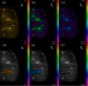

Fig. 9

Segmented FLIM image of short component [Fig. 8b] was composed of the three fluorescence lifetimes that were experimentally measured for (b), (c), and (d) masks projected on the sample (a). The experimental decays measured while the sample was exposed to these spatial patterns are compared with the distribution of fluorescence lifetimes obtained in raster-scanning and fitting (rapid-double algorithm) mode [Fig. 8e] for the same region in the sample (a).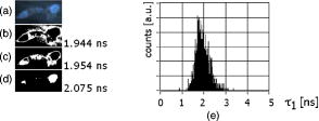

5.

Discussion

The main goal of GIP calculations is to provide a fitting algorithm with reliable phenomenological parameters to reduce the number of fitting iterations and improve FLIM imaging throughput. However, the main drawback of the traditional approaches (Table 1) is the lack of the correspondence between how the GIPs are acquired (e.g., in the quadrant average manner) and the actual morphology or photobiochemical structure of the sample. Although segmentation based on a white-light image has been presented in the context of a GA approach,²⁵ the implementation was effectively manual and thus could be improved by an automated, less subjective treatment of the bright field intensity. Nevertheless, it would seem more appropriate to employ fluorescence-based image segmentation for FLIM preprocessing rather than a white-light or morphology approach. This is because a correspondence exists between fluorescence intensity (measured with, for example, a color CCD camera) and the photophysical properties of the fluorophores (measured as fluorescence spectrum or fluorescence lifetimes).

One disadvantage of using a fluorescence image for segmentation is the fact that during wide-field imaging, the detector gathers out-of-focus fluorescence, leading to fluorescence image blurring and as a consequence degrades the quality of the segments. This could be avoided by using raster-scanned datasets for segmentation, but at a significant cost in terms of time. Another solution would be to use excitation light sectioning for improving the spatial resolution of fluorescence images, as already demonstrated in non-DMD³¹ and DMD^{12, 13} based optical microscopy setups.

In the context of the work of Verveer, Squire, and Bastiaens,²⁷ it is important to improve the SNR to gain reliable GIPs for further analysis of poor SNR individual datasets. Software binning accumulates both signal and noise and requires dedicated steps to remove the background. Hardware binning generally improves SNR by default and gives better results than SB. More importantly, however, HB better exploits the dynamic range of the detector and acquisition board and significantly reduces the time required to establish GIPs. While HB with a DMD spatial illuminator requires only one measurement per segment and avoids signal collection from nonfluorescent sample regions, SB requires “blind” collection of large datasets without knowledge of which data are actually useful. Therefore, in comparison to off-line data analysis, preprocessing by means of fluorescence image segmentation seems to be a significant improvement in terms of speed and accuracy of high-content studies.

During segmented fluorescence lifetime acquisition and GIPs estimation, besides the decay constants, many other coefficients (e.g., fluorescence intensity, relative intensities of the components, background, total photon counts, etc.) can be extracted and stored. Moreover, the model decay curve itself can be generated and stored. Due to the spatial correspondence between the steady-state fluorescence intensity with phenomenological parameters, individual adjustments to, for example, acquisition time can be performed for every pixel to optimize SNR or to improve the dynamic range of the photodetector. A similar approach, developed originally to reduce photobleaching of biological samples, was recently proposed by Hoebe ³² and was realized by modifying a confocal scanning microscope with an acousto-optic modulator. The photon counts were continuously monitored and the exposure time was reduced in proportion to the fluorescence intensity by actively reducing the excitation light intensity. In our adaptive approach, the photodetection dwell time is directly controlled. Therefore, the acquisition time can be shortened or lengthened depending on the fluorescence intensity, thus maintaining a consistent SNR and effectively extending the dynamic range of detection.

In the preprocessing algorithm presented in Sec. 3.4, the color fluorescence image [Fig. 5a] was used to perform hue-based [Fig. 5b] segmentation to spectrally and spatially distinguish between regions that contain different fluorophores [Figs. 5c and 5d]. Further intensity-based segmentation within respective hue segments was performed (Fig. 6) to account for issues such as nonhomogeneous illumination. Looking at the result presented in Fig. 7b, one can notice some fluorescence lifetime variations across the FLIM image. This is due to the fact that the least-square goodness-of-fit estimators used together with low photon counts delivered intensity dependent values of fluorescence lifetimes.²⁹ Nevertheless, opposite to standard stead-state wide field fluorescence imaging, the output FLIM image was less susceptible to experimental conditions and exhibited better contrast between the two sample regions.

As illustrated in Fig. 4, a satisfactory level of precision and accuracy could only be obtained with the double exponential decay model when the IRF was taken into account. With this approach, the accuracy was equal to $⟨A⟩∕A=1.01$ , $⟨{\tau }_1⟩∕{\tau }_1=1.01$ , and $⟨{\tau }_2⟩∕{\tau }_2=1.04$ while the standard deviation was smaller than 0.02. Although the rapid algorithm was fast and supplied reasonable ${\chi }^2$ values, the calculated accuracy was equal to $⟨A⟩∕A=0.88$ , $⟨{\tau }_1⟩∕{\tau }_1=1.10$ , and $⟨{\tau }_2⟩∕{\tau }_2=1.17$ . Fitting the decaying part of the experimental curve (without considering the IRF) delivered decay components relatively fast and accurately ( $⟨{\tau }_1⟩∕{\tau }_1=1.00$ , $⟨{\tau }_2⟩∕{\tau }_2=1.01$ ), although the accuracy in calculating the fraction parameter was poor $(⟨A⟩∕A=0.84)$ .

Although being accurate, the double IRF modeling was much slower in comparison to less accurate methods, and therefore is usually associated with low throughput in FLIM imaging. This is mostly due to the application of time-consuming iterative convolution-based fitting that is required when IRF is accounted for in detailed and quantitative studies. With a customized LabVIEW Levenberg-Marquard fitting function, the typical calculation time obtained was equal to $987\pm 90\mathrm{ms}$ and $43\pm 1.6\mathrm{ms}$ , respectively, for fitting with and without considering the IRF. When GIPs were supplied, the calculation time was reduced to $609\pm 67$ and $40\pm 5\mathrm{ms}$ , respectively. Additionally, the analysis time for the double IRF method strongly depended on the number of experimental datapoints due to the convolution between the theoretical decay model and the IRF function performed in every iteration. The ${\chi }^2∕N$ $\left({\chi }^2\right)$ was found to be $0.27\pm 0.05$ (54.6) and $0.09\pm 0.01$ (18.2) for respective cases, and no noticeable change in ${\chi }^2$ values was observed whether GIPs were supplied or not. The rapid double decay lifetime determination algorithm required only $0.29\text{-}\mathrm{ms}$ calculation time and resulted in ${\chi }^2∕N$ $\left({\chi }^2\right)=0.14\pm 0.06$ (27.8). The ${\chi }^2∕N$ obtained for the rapid double algorithm was apparently smaller or comparable to the results obtained with the fitting algorithms. However, when the initial coefficients for the first iteration of the double IRF algorithm were fixed to $A=0.705$ , ${\tau }_1=0.549$ , and ${\tau }_2=2.925$ , as obtained with rapid double method, the ${\chi }^2∕N$ $\left({\chi }^2\right)$ increased to 9.3 (1936). This suggests that the analysis of only the decaying part of the fluorescence lifetime (as is the case for double and rapid double algorithms) underrated the value of the short component and its contribution to the whole experimental dataset. Additionally, the absolute values of the rapid algorithm output varied with the time window used to select the decaying part of the experimental dataset. Therefore, it is questionable whether rapid fluorescence estimation algorithms are reliable enough for raster-scanned data segmentation.

When the linear approach extended the double IRF fitting procedure, the $I_m^i\left(t\right)$ dataset corresponding to a given segment was restored directly from the reference table. Around $5.8\mu \mathrm{s}$ (50 times less than for the rapid double algorithm) was required to verify whether the set of initial coefficients $T_{S(x,y)}$ accurately modeled the experimental dataset or not. The advantage of using GIPs and the linear approach is particularly obvious when arduous calculations (i.e., time-consuming model generation based on reliable GIPs) are performed before actual on-line pixel-by-pixel data analysis. The off-line data analysis (with e.g., time invariant global decay analysis) is also possible when software binning is performed on the unprocessed FLIM datasets.

Traditionally, time-domain FLIM image reconstruction is performed pixel by pixel or by using global algorithms. For demonstration purposes, we have used raster-scanned sequential decay analysis and image reconstruction [Fig. 3a]. However, the DMD-based spatial illuminator provides the additional possibility to access any ROI on the sample by switching on the groups of corresponding micromirrors. Owing to that feature, therefore, another new and interesting imaging modality has been demonstrated. Segmented FLIM imaging basically visualizes the fluorescence lifetime coefficients intended to be GIPs for further eventual adjustments, as ultimate values that need no further optimization. A SFLIM approach may only be appropriate for certain functional imaging applications. For example, the SFLIM may be suitable to discriminate between multiple fluorophores with overlapping emission spectra, but would not be useful to determine the molecular environment of the fluorophore. In the first case, qualitative differences between these few spectrally overlapping dyes are mapped on the sample, and fluorescence lifetimes are measured in respective sample segments to provide better contrast and potentially deliver quantitative information. Assuming the homogeneity of illumination and insensitivity of the fluorophore to its environment, which is true for quantum dots and many other fluorochromes, we may conclude that SFLIM is able to provide fast FLIM image previewing to study spatial distribution and relative concentration of fluorescent dyes in multiplexed systems. In the second case, since the hue-intensity-based segmentation is susceptible to dye concentration, illumination homogeneity, and local microenvironment, the fluorescence intensity of diluted but unquenched dye can be easily mismatched with high-concentration high-quenching cases. In this case, the SFLIM may not be sufficiently resolvable to reconstruct microenvironment variations.

To compare DMD raster-scanned FLIM images with the segmented FLIM approach, we have selected and measured the same sample region with the two techniques. The fraction parameter $A$ [Fig. 8d], obtained with the rapid double exponential model, applied to the raster-scanned datasets approaches a value of 1 and the long component is quasi-randomly distributed. Most probably this is due to low total photon counts encountered during raster scanning, and suggests that a single decay model could be sufficient to provide reasonable results. This is not the case for SFLIM analysis [Fig. 8a], which demonstrates $A$ approaching a value of 0.85 and a long component measured at the nucleus site equal to $5.70\mathrm{ns}$ . The long component is thus observed only for SFLIM and demonstrates that the SNR has been improved in comparison to the raster-scanning case. The origin of this long component is presently unknown to us. The average values of short decay components are around 2.1 and $1.9\mathrm{ns}$ , as measured for SFLIM and FLIM, respectively, and are slightly lower than the literature data for Hoechst dye $\left(2.2\text{to}2.3\mathrm{ns}\right)$ . Since we did not store the experimental decay datasets but rather saved the decay coefficients as a color image directly, the scales for the ${\tau }_1$ and ${\tau }_2$ images in Fig. 8 differ. Nevertheless, the absolute values (at least for ${\tau }_1$ ) correspond in both SFLIM and FLIM cases. This is visualized in Fig. 9, where the short fluorescence lifetime component measured for the three segments [Figs. 9b, 9c, 9d] covering the region of interest compare well with the decay distribution observed for the raster-scanned case [Fig. 9e].

To judge if the three-step algorithm presented here is justified or maybe off-line data preprocessing is sufficient for improvement of GIP estimation and data management, three different scenarios can be considered. In the first one, following “blind” raster scanning that is subject to poor SNR, the rapid lifetime estimation algorithm is applied to establish sample segments that exhibit similar decay properties. Next, off-line accumulation of the fluorescence lifetime histograms within the segments is performed to further estimate GIPs for more detailed pixel-by-pixel or global data analysis. Although attractive, it is questionable to use the first scenario for complex systems like double exponential decay imaging. The rapid estimation algorithms may not be reliable enough to define segments properly and to group identical fluorophores to further estimate GIPs. However, rapid lifetime estimation for GIP assessment performed on the pixel-by-pixel bases seems to be reasonable.

In the second scenario, wide-field fluorescence image is acquired prior to raster scanning to perform sample segmentation. However, the fluorescence decay dataset accumulation is performed off-line with SB on the set of blindly collected fluorescence signals. The segmentation step is followed by more detailed off-line pixel-by-pixel or global analysis exploiting the GIPs. This approach is justified and recommended for biological systems to limit photobleaching. When the photodamage is not a critical issue, hardware binning is preferable for GIPs estimation, as in the third scenario described before. Due to the reliability of the GIP parameters estimated in the preprocessing step, the approach offers more rapid data analysis, a better SNR, and ultimately more accuracy, as well as the ability to provide the results on-line. Adaptive FLIM image reconstruction is performed by exploiting all the preprocessed information. The DMD-based spatial illuminator is flexible enough to perform any of the described scenarios with no optical system rearrangements. Global analysis algorithms can be easily adapted off-line, with the advantage for initial fitting parameters to be informed by GIP established in relation to functional/morphological sample structure.

6.

Conclusions

We propose a new approach to FLIM imaging based on good initial global fitting parameters estimation. The estimation relies on the averaged hardware-binned fluorescence signal from disjointed or contiguous segments of a sample. The segments are semiautomatically designed based on division of the hue/intensity histograms of the color fluorescence image of the sample. Segments prepared like this allow us to selectively photoexcite the regions of the sample exhibiting similar spectral properties. The fluorescence lifetimes are recorded and analyzed for the entire collection of the segments and serve as a set of good initial fitting parameters for further raster scanning and more detailed on-line data analysis.

Additionally, we demonstrate the improvement in FLIM data analysis time without compromising the accuracy or precision in extracting the fluorescence decay phenomenological coefficients. The improvement is achieved because the heaviest computational work to estimate GIPs and respective decay models is performed in the data preprocessing step. During FLIM reconstruction, an on-line computationally efficient validation of the model and further optional fitting is performed rather then blind data analysis.

Additionally, when a sufficient number of segments is designed, the GIPs calculated in the preprocessing step of the presented algorithm become the final decay coefficients, with no need for further optimization. The segmented FLIM image is therefore obtained in a rapid manner, by the acquisition and analysis of only a very limited number of fluorescence decay curves.

We demonstrate that the presented algorithm combined with a DMD-based spatial illuminator offers a lot of flexibility in FLIM data acquisition and management, opposite of spatial and photophysical constrains of traditional global data processing. The implications of our approach in terms of fitting accuracy are substantial for many biological studies including FRET, redox state imaging, or high content imaging.