2.1.

Forward Model

The diffusion equations were solved by Kienle ³ using the Fourier transform approach for a two-layer turbid medium with a semi-infinite second layer. We directly adopted this method for tomographic imaging and a brief description of the analytical solution is given here for the sake of completeness. A two-layer turbid medium is considered with upper layer thickness $l$ and a semi-infinite second layer. An infinitely thin beam of frequency-modulated light is incident perpendicular on the top surface of a two-layer turbid medium. The beam is scattered isotropically at the depth of $z_0={({\mu }_{a1}+{\mu }_{s1}^{\prime })}^{-1}$ , where the ${\mu }_{a1}$ and ${\mu }_{s1}^{\prime }$ are the absorption and reduced scattering coefficients of the first layer, and $z_0$ is in the range of $1\text{to}2\mathrm{mm}$ for typical background breast-tissue absorption and scattering properties. The diffusion equation for the photon density wave at two layer structure is given as

The diffusion equations were first transformed to ordinary differential equations with the use of a 2-D Fourier transform

The fluence rate in the spatial domain $(x,y,z)$ can be obtained by spatial Fourier inversion:

2.2.

Image Reconstruction Using Two-Layer Tissue Model

In the Born approximation, the photon density wave originating from a source at $r_s$ and measured inside the tissue at $r$ , is a linear superposition of its incident ${\Phi }_0$ (homogeneous) and the scattered ${\Phi }_{\mathrm{sc}}$ (heterogeneous) parts given as $\Phi (r_s,r,\omega )={\Phi }_0(r_s,r,\omega )+{\Phi }_{\mathrm{sc}}(r_s,r,\omega )$ . By using the first-order solution to the heterogeneous equation under the approximation that ${\Phi }_{\mathrm{sc}}(r_s,r,\omega )⪡{\Phi }_0(r_s,r,\omega )$ , we obtain ${\Phi }_{\mathrm{sc}}(r_d,r_s,\omega )=-(1∕D_0)\int G(r,r_d,\omega )\Delta {\mu }_a\left(r\right){\Phi }_0(r_s,r,\omega )d^{3}r$ , where $r_d$ represents detector position, $G(r,r_d,\omega )$ represents the scattered field at $r_d$ due to the point scattered at $r$ , $\Delta {\mu }_a\left(r\right)$ is the change of absorption coefficient at voxel at location $r$ , and $D_0$ is the diffusion coefficient of the homogeneous medium. Figure 1 illustrates the source position $r_s$ , field point $r$ , detector position $r_d$ , and $\rho$ used for computing the incident field.

Fig. 1

Configuration for simulations and reconstructions.

When using the two-layer model, ${\Phi }_0(r_s,r,\omega )$ is calculated based on the depth of the voxel to which the fluence is being computed. For voxels in the three regions the fluence rates are represented by ${\Phi }_{00},{\Phi }_{01}$ , and ${\Phi }_{02}$ , and $D_0$ is replaced by $D_1$ or $D_2$ , depending on the voxel location in the layered structure. The Green function $G(r,r_d,\omega )$ of the homogeneous equation at the detector $r_d$ is given as $G(r,r_d,\omega )=(D_i∕S){\Phi }_0(r,r_d,\omega )={\Phi }_i\{{[{(x_d-x)}^2+{(y_d-y)}^2]}^{1∕2},z,\omega \}$ , which could be calculated again using spatial Fourier inversion from any one of Eq. 8 (if voxel depth $z<z_0$ ), Eq. 9 (if voxel depth $z_0⩽z<l$ ), and Eq. 10 (if $z⩾l$ ), depending on the voxel depth from the surface.

The dual-zone mesh scheme introduced by us earlier¹⁶ was used to segment the imaging volume into lesion and background regions designated as $L$ and $B$ , respectively. The weight matrix is calculated using the two-layer model as ${\left[{\mathsf{U}}_{sd}\right]}_{M\times 1}={[{\mathsf{W}}_L,{\mathsf{W}}_B]}_{M\times N}{[{\mathsf{M}}_L,{\mathsf{M}}_B]}^T$ , where ${\mathsf{W}}_L={[-G(r_{vj},r_{di}){\Phi }_0(r_{si},r_{vj})∕D_l]}_{M\times N_L}$ and ${\mathsf{W}}_B={[-G(r_{vk},r_{di}){\Phi }_0(r_{si},r_{vk})∕D_l]}_{M\times N_B}$ are weight matrices for lesion and background volumes, respectively; $\left[M_L\right]=[{\int }_{1_L}\Delta {\mu }_a\left(r^{\prime }\right)d^3{r}^{\prime },\mathrm{\dots },{\int }_{N_L}\Delta {\mu }_a\left(r^{\prime }\right)d^3{r}^{\prime }]$ and $\left[M_B\right]=[{\int }_{1_B}\Delta {\mu }_a\left(r^{\prime }\right)d^3{r}^{\prime },\mathrm{\dots },{\int }_{N_B}\Delta {\mu }_a\left(r^{\prime }\right)d^3{r}^{\prime }]$ are the total absorption distributions of lesion and background volumes, respectively; and $D_l$ equals $D_1$ or $D_2$ , depending on the voxel location in the layered structure. The dual-zone mesh scheme significantly reduces the total number of voxels with unknown optical properties and dramatically improves the convergence of inverse mapping of target optical properties.^{16, 17}

3.1.

Simulations

The imaging reconstruction algorithm developed in Sec. 2 was validated using forward data generated by the finite-element method (FEMLAB 6.2). The source-detector geometry is shown in Fig. 2 . There are total of nine sources and 10 detectors. The middle slot was used for a commercial ultrasound transducer. The geometry used in simulation was the same as that used in phantom and clinical measurements.

Fig. 2

Probe geometry. The red stars are sources, and the blue circles are the detectors. The middle slot is for a commercial ultrasound transducer. (Color online only.)

Two sets of simulations were performed. In the first set of simulations, a spherical target of $1\mathrm{cm}$ diameter was embedded in the layered structure at a $1.5\text{-}\mathrm{cm}$ depth from the surface. The target center was placed at $0.9\mathrm{cm}$ , and its absorption coefficient was varied from $0.07\text{to}0.30{\mathrm{cm}}^{-1}$ . Forward data was generated from two-layer structures whose optical properties were in the range of typical breast tissue and chest wall. For each set of target data, a reference data set was also generated using the same layered structure with no target in the medium. Perturbation data were used for imaging reconstruction of the target. Two sets of imaging reconstructions were performed. One set of images was reconstructed from known optical properties of the two-layer structure, while another set was obtained by using fitted optical properties from the reflectance data. The reconstruction results for the first set provided the ideal condition when no fitting error for the two-layer optical properties was considered. The second reconstruction set is relevant to realistic clinical experiments, where the first- and second-layer optical properties must be estimated from the reflectance measurements. For this set of simulations, image reconstruction was also performed by using a semi-infinite model and a two-layer model with true background optical properties and fitted background properties.

In the second set of simulations, the absorption coefficient of the $1\text{-}\mathrm{cm}$ -diam target was fixed at $0.2{\mathrm{cm}}^{-1}$ and the second-layer background optical absorption was varied from $0.02\text{to}0.15{\mathrm{cm}}^{-1}$ at $0.03\text{-}{\mathrm{cm}}^{-1}$ intervals to simulate a range of chest-wall optical absorptions. For each set of background optical properties, forward data were generated with and without target. Image reconstruction was performed by using known background optical properties and fitted background optical properties. This set of simulations was intended to evaluate the effect of fitting error on reconstructed target absorption.

3.2.

Phantom and Clinical Experiments

The experimental validation of the imaging algorithm was performed using an existing frequency-domain near-IR (NIR) system.¹⁹ It consisted of laser diodes of 780- and $830\text{-}\mathrm{nm}$ wavelengths. The outputs of the laser diodes were amplitude modulated at $140\mathrm{MHz}$ and optically switched to nine positions on a hand-held probe. Ten optical fibers of $3\mathrm{mm}$ diameter were coupled to 10 parallel detection channels. Solid silicone phantoms were used to emulate the second layer over which intralipid solution was used for the top layer. All the phantom experiments were performed using a flat interface between the layers. The measurements were first made on simple two-layer structures with various layer depths and used as the reference data. The measurements were repeated for the same structures with solid target phantoms immersed in the intralipid layer at known depths. Two types of target phantoms were used; one with low absorption to emulate a benign lesion and one with a high absorption to emulate a cancerous lesion in the breast.^{20, 21} The layer thickness, target position, and target size were known in these phantom measurements as opposed to the clinical cases were we would estimate these parameters using a coregistered ultrasound probe.

The imaging algorithm was demonstrated with clinical examples. The study protocol was approved by a local Institutional Review Board (IRB) committee. Signed informed consent was obtained from all patients who agreed to participate in the study. In clinical experiments, NIR optical source fibers, detector fibers, and a commercial ultrasound transducer were integrated on a handheld probe.¹⁹ Patients were scanned in a supine position, while multiple sets of optical reflectance measurements were made with coregistered ultrasound images at lesion locations and symmetric locations of the contralateral normal breast. The measurements obtained at normal locations were used to estimate background optical properties, which were used to compute a weight matrix for imaging.

3.3.

Estimation of Two-Layer Optical Properties and Image Reconstruction

Two-layer optical properties were estimated from fitting reflectance measurements made on the layered structure to analytical solution using the Nelder-Mead simplex algorithm as described in our previous paper.¹² This algorithm minimizes a scalar-valued nonlinear function of multiple independent parameters by using only the function values, and it is chosen due to its simplicity and good convergence in spite of the slow convergence rate. We chose various initial values and found that initial values are not critical as long as the function converges. For each case, the initial values were chosen as 0.05, 5.0, 0.05, and $5.0{\mathrm{cm}}^{-1}$ for ${\mu }_{a1}$ , ${\mu }_{s1}^{\prime }$ , ${\mu }_{a2}$ , and ${\mu }_{s2}^{\prime }$ , respectively. In the phantom and clinical experiments, the thickness of the upper layer was estimated by using the coregistered ultrasound image. The nonlinear regression routine used here, fminsearch, is available in MATLAB.

In simulations, the voxel size was chosen as $0.1\mathrm{cm}$ in the $x$ and $y$ dimensions for fine mesh and $1.5\mathrm{cm}$ for coarse mesh. The corresponding voxel sizes were 0.25 and $1.5\mathrm{cm}$ in phantom studies, and 0.5 and $1.5\mathrm{cm}$ for clinical data. In all experiments, the voxel size in depth was $0.5\mathrm{cm}$ in the fine-mesh zone and $1.5\mathrm{cm}$ in the coarse-mesh zone. The choice of fine-mesh size is based on SNR and also spatial sampling considerations. The fine-mesh volume for all experiments was chosen at least 2.5 times larger than the target size and centered at the target position. Clinical experiments were performed by fitting the two-layer optical properties of the contralateral breast using the layer depth provided by coregistered ultrasound images. In all experiments, the dual-mesh algorithm was used for inversion with either known target location or size in simulation and phantom experiments or a priori information provided by coregistered ultrasound in clinical experiments.

4.1.

Simulation

In the first set of simulations, targets of various absorption properties were embedded in a layered structure of $1.5\mathrm{cm}$ upper layer thickness. The first and second layer known optical properties were ${\mu }_{a1}=0.02{\mathrm{cm}}^{-1}$ and ${\mu }_{s1}^{\prime }=7.0{\mathrm{cm}}^{-1}$ and ${\mu }_{a2}=0.10{\mathrm{cm}}^{-1}$ and ${\mu }_{s2}^{\prime }=7.0{\mathrm{cm}}^{-1}$ , respectively. The target absorption coefficients were chosen as 0.07, 0.10, 0.15, 0.20, 0.25, and $0.30{\mathrm{cm}}^{-1}$ , and the reduced scattering coefficient was kept at $7.0{\mathrm{cm}}^{-1}$ . Reference data were also generated for the two-layer structure in the absence of the target. Figure 3 shows an example of reconstructed target absorption maps of an absorber ( ${\mu }_a=0.30{\mathrm{cm}}^{-1}$ and ${\mu }_s^{\prime }=7.0{\mathrm{cm}}^{-1}$ ) embedded in the layered-medium when the known optical properties were used in the reconstruction. Figure 3a shows the reconstruction result of using a semi-infinite model for the two-layer structure and known first-layer background values of ${\mu }_{a1}=0.02{\mathrm{cm}}^{-1}$ and ${\mu }_{s1}^{\prime }=7{\mathrm{cm}}^{-1}$ . Figure 3b shows the two-layer-model reconstruction using known two-layer background values of ${\mu }_{a1}=0.02{\mathrm{cm}}^{-1}$ , ${\mu }_{s1}^{\prime }=7.0{\mathrm{cm}}^{-1}$ , ${\mu }_{a2}=0.10{\mathrm{cm}}^{-1}$ , and ${\mu }_{s2}^{\prime }=7.0{\mathrm{cm}}^{-1}$ . The reconstructed maximum absorption values were $0.186{\mathrm{cm}}^{-1}$ (62%) and $0.220{\mathrm{cm}}^{-1}$ (73%), respectively. About 11% improvement in reconstruction accuracy was achieved using the layer-based reconstruction under this ideal scenario. When using a semi-infinite model to fit background optical properties of the two-layer structure, ${\mu }_a=0.069{\mathrm{cm}}^{-1}$ and ${\mu }_s^{\prime }=5.94{\mathrm{cm}}^{-1}$ were obtained. Figure 4a shows the result of semi-infinite-model-based reconstruction and the reconstructed maximum absorption coefficient was $0.242{\mathrm{cm}}^{-1}$ [Fig. 4a]. When fitted two-layer optical properties of ${\mu }_{a1}=0.037{\mathrm{cm}}^{-1}$ , ${\mu }_{s1}^{\prime }=7.24{\mathrm{cm}}^{-1}$ , ${\mu }_{a2}=0.10{\mathrm{cm}}^{-1}$ , and ${\mu }_{s2}^{\prime }=5.09{\mathrm{cm}}^{-1}$ were used in two-layer-model-based reconstruction, the reconstructed maximum absorption coefficient was $0.2613{\mathrm{cm}}^{-1}$ [Fig. 4b]. About 7% improvements in reconstruction accuracy were achieved even with fitting errors of the two-layer optical properties.

Fig. 3

Image reconstruction results using true background optical properties obtained using (a) a semi-infinite model for the two-layer structure and (b) a two-layer model for the layered structure. In each figure, the first slice is the spatial $x\text{-}y$ image at a $0.5\text{-}\mathrm{cm}$ depth from the surface and the last slice is at a $3.0\text{-}\mathrm{cm}$ depth. The dimension of each slice is $8\times 8\mathrm{cm}$ and the spacing between the slices is $0.5\mathrm{cm}$ . The vertical scale is absorption coefficient in inverse centimeters.

Fig. 4

Image reconstruction results using fitted background optical properties obtained using (a) the semi-infinite model with the fitted background optical properties and (b) the two-layer model with fitted background optical properties. In each figure, the dimension of each slice is $8\times 8\mathrm{cm}$ and the spacing between the slices is $0.5\mathrm{cm}$ . The vertical scale is absorption coefficient in inverse centimeters.

Figure 5 shows the reconstructed maximum absorption coefficient versus true target absorption value with known and fitted optical properties of two-layer model (black star and purple cross lines) and the semi-infinite approximation for the layered structure (green triangle and red square lines), respectively. It is interesting to note that the two-layer model improves the reconstruction accuracy only at higher contrast end when known optical properties of two-layers are used. This is due to the use of a more accurate weight matrix for the two-layer structure. Because both semi-infinite and two-layer models use the linear Born approximation, the reconstructed target absorption is reduced at higher contrast. When the fitted two-layer optical properties are used, the improvement is distributed at both high and low contrast. The improvement at low contrast is due to the use of more accurate first-layer background properties. Because reconstructed target ${\mu }_a={\mu }_{a1}+\text{reconstructed}$ $\Delta {\mu }_a$ , a higher fitted background absorption using the semi-infinite model yields a higher target ${\mu }_a$ compared with using the two-layer model. This problem is less pronounced when the target to background ratio is higher.

Fig. 5

Comparison of target absorption coefficients obtained with a semi-infinite-model-based reconstruction for the layered structure (green triangle line: using true background values; red squares: using fitted background values) and a two-layer-model based reconstruction for the layered structure (black stars: using true background values; purple crosses: using fitted background values). The blue circle line is the true target absorption coefficient. (Color online only.)

In the second set of simulations, the first layer optical properties and the second layer reduced scattering coefficient were fixed at ${\mu }_{a1}=0.02{\mathrm{cm}}^{-1}$ , and ${\mu }_{s1}^{\prime }=7{\mathrm{cm}}^{-1}$ , and ${\mu }_{s2}^{\prime }=7{\mathrm{cm}}^{-1}$ . However, the second layer background ${\mu }_{a2}$ was varied from $0.02\text{to}0.15{\mathrm{cm}}^{-1}$ to simulate a range of chest-wall absorption. Table 1 lists the true and fitted two-layer optical properties and the corresponding reconstructed maximum target absorption coefficient. Target reconstruction results using true and fitted background properties for each set of background values are within 13%. The small difference results from the fitting error of first-layer ${\mu }_{a1}$ .

Table 1

Simulation results using the semi-infinite model and the two-layer model with fitted background values. Target center depth C=0.9 cm. Target radius R=0.5cm. Second layer depth D=1.5 cm. Refractive index (n 1=1.33, n 2=1.4).

4.2.

Phantom Experiments

Phantom experiments were performed with various upper layer thicknesses and two $1\text{-}\mathrm{cm}$ diameter spherical targets of high absorption (phantom 1) and low absorption (phantom 2) coefficients located at various depths. The calibrated absorption and reduced scattering coefficients obtained from the same phantom materials were ${\mu }_a=0.23{\mathrm{cm}}^{-1}$ and ${\mu }_s^{\prime }=5.45{\mathrm{cm}}^{-1}$ for phantom 1 and ${\mu }_a=0.07{\mathrm{cm}}^{-1}$ and ${\mu }_s^{\prime }=5.50{\mathrm{cm}}^{-1}$ for phantom 2 at $780\mathrm{nm}$ . The upper layer was intralipid solution of measured optical properties ${\mu }_a=0.022{\mathrm{cm}}^{-1}$ and ${\mu }_s^{\prime }=7.2{\mathrm{cm}}^{-1}$ , and the bottom layer comprised silicon phantoms of measured optical properties ${\mu }_a=0.06{\mathrm{cm}}^{-1}$ and ${\mu }_s^{\prime }=15{\mathrm{cm}}^{-1}$ (silicon phantom 1) and ${\mu }_a=0.12{\mathrm{cm}}^{-1}$ and ${\mu }_s^{\prime }=15{\mathrm{cm}}^{-1}$ (silicon phantom 2).

The reconstruction results were obtained by using fitted two-layer optical properties from the reflectance measurements. The results of six different experiments of phantoms 1 and 2 are tabulated in Tables 2, 3 . The reconstruction accuracy calculated from the calibrated target values using the semi-infinite and two-layer models are also given in the tables. For the low-contrast phantom 2, because the two-layer model provides more accurate background value, the reconstructed absorption coefficient is greater than 80% more accurate than that obtained from the semi-infinite model at a shallow depth, such as $1.5\mathrm{cm}$ . For the high-contrast phantom 1, the improvement of 10 to 20% is obtained when the two-layer analytic solution is used instead of the semi-infinite model. As expected, the difference in reconstructed values between the two models reduces as the layer depth increases. Because second-layer optical properties mainly affect distance measurements acquired at longer source-detector pairs and these measurements have lower SNRs compared with shorter pairs, the fitted optical properties of the second layer are less accurate than those of the first layer. However, the reconstructed target contrast is not very sensitive to the second layer properties.

Table 2

Reconstruction results for phantom 1 ( μa=0.23cm−1 and μs′=5.45cm−1 ) using the semi-infinite model and the two-layer model with fitted background values.

Table 3

Reconstruction results for phantom 2 ( μa=0.07cm−1 and μs′=5.50cm−1 ) using the semi-infinite model and the two-layer model with fitted background values.

An example of imaging results of phantom 1 using silicon phantom 1 as the second layer is given in Figs. 6 and 7 . Figure 6 shows the fitted background optical properties of ${\mu }_{a1}$ , ${\mu }_{s1}^{\prime }$ , ${\mu }_{a2}$ , and ${\mu }_{s2}^{\prime }$ versus iterations when the first layer depth is $2.4\mathrm{cm}$ (third line in Table 1 two-layer model). The fitting procedure converges and the fitted background values at iteration of 272 are ${\mu }_{a1}=0.027{\mathrm{cm}}^{-1}$ , ${\mu }_{s1}^{\prime }=9.90{\mathrm{cm}}^{-1}$ , ${\mu }_{a2}=0.041{\mathrm{cm}}^{-1}$ , and ${\mu }_{s2}^{\prime }=18.53{\mathrm{cm}}^{-1}$ .

Fig. 6

Phantom experiments of fitted background optical properties versus iteration. Intralipid was used as the first layer and the silicon phantom 1 was used as the second layer. The depth of the intralipid layer was $2.4\mathrm{cm}$ . The measured optical properties of Intralipid were ${\mu }_a=0.022{\mathrm{cm}}^{-1}$ and ${\mu }_s^{\prime }=7.2{\mathrm{cm}}^{-1}$ , and those of the silicon phantom 1 were ${\mu }_a=0.06{\mathrm{cm}}^{-1}$ and ${\mu }_s^{\prime }=15{\mathrm{cm}}^{-1}$ . (a) and (c) Fitted layer absorption coefficient versus iteration for first and second layers, respectively, and (b) and (d) fitted reduced scattering coefficient versus iteration for first and second layers, respectively.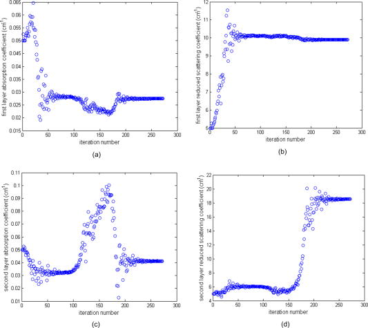

Fig. 7

Reconstructed absorption maps of phantom 1 placed in Intralipid layers of 0.9, 1.5, and $1.8\mathrm{cm}$ depth. The second layer silicon phantom was located at 1.5, 2.1, and $2.4\mathrm{cm}$ depth, respectively. (a) and (b), The target center was located at $0.9\mathrm{cm}$ depth. The first slice is the spatial $x\text{-}y$ image of $8\times 8\mathrm{cm}$ obtained at a $0.4\text{-}\mathrm{cm}$ depth, and the second and third slices at 0.9 and $1.4\mathrm{cm}$ , respectively. (c) and (d) The target center was located at a $1.5\text{-}\mathrm{cm}$ depth. The first slice is the spatial $x\text{-}y$ image of $8\times 8\mathrm{cm}$ obtained at a $0.5\text{-}\mathrm{cm}$ depth, and the second and third cross sections at 1.0 and $1.5\mathrm{cm}$ , respectively. (e) and (f). The target center was located at a $1.8\text{-}\mathrm{cm}$ depth. The first slice is the spatial $x\text{-}y$ image of $8\times 8\mathrm{cm}$ obtained at a $0.3\text{-}\mathrm{cm}$ depth, and the fourth cross-section slice is at a $1.8\text{-}\mathrm{cm}$ depth. (a), (c), and (e) Reconstructed absorption maps obtained at $780\mathrm{nm}$ using fitted background values and a semi-infinite model for the layered structure. Reconstructed target maximum absorption coefficients were 0.158, 0.169, and $0.191{\mathrm{cm}}^{-1}$ , respectively. (b), (e), and (f) Reconstructed absorption maps obtained at the same wavelength using the two-layer model with fitted background values. The reconstructed target maximum absorption coefficients were 0.201, 0.206, $0.198{\mathrm{cm}}^{-1}$ , respectively.

Figure 7 shows the absorption maps of high-contrast phantom 1 placed in Intralipid layers of 0.9-, 1.5-, and $1.8\text{-}\mathrm{cm}$ depth. The second layer (silicon phantom 1) was located at 1.5-, 2.1-, and $2.4\text{-}\mathrm{cm}$ depths, respectively. Figure 7a, 7c, 7e show reconstructed absorption maps obtained at $780\mathrm{nm}$ using a semi-infinite model for the layer structure. Reconstructed target maximum absorption coefficients were 0.158 (68%), 0.169 (73%), and 0.191 (83%) ${\mathrm{cm}}^{-1}$ , respectively. Figures 7b, 7d, 7f show reconstructed absorption maps obtained at the same wavelength using the two-layer model. The reconstructed target maximum absorption coefficients were 0.201 (88%), 0.209 (91%), and $0.198{\mathrm{cm}}^{-1}$ (86%), respectively. About 3 to 20% improvement in reconstruction accuracy was obtained in this set of experiments. The reconstruction results obtained at $830\mathrm{nm}$ are very similar to the results at $780\mathrm{nm}$ . Therefore, images of $830\mathrm{nm}$ are not shown here.

4.3.

Clinical Experiments

The two-layer-model-based reconstruction was demonstrated using clinical data. Two examples of benign and malignant cases are given here to demonstrate the potential of this new reconstruction technique. Figure 8 shows the ultrasound image from the normal contralateral site [Fig. 8a] and lesion site [Fig. 8b] of a $54\text{-}\text{year}$ -old patient. The lesion was approximately $0.8\mathrm{cm}$ deep with approximately $0.3\mathrm{cm}$ radius in the $z$ direction (depth) and the lateral radius or shape of the lesion was approximately $1.0\mathrm{cm}$ , as seen in the ultrasound image. We can see from Fig. 8a that the upper layer thickness is about $1.4\mathrm{cm}$ with an almost flat interface between the chest wall and the breast tissue. The fitted optical properties of the breast and chest-wall layer from the contralateral site with no lesion were ${\mu }_{a1}=0.041{\mathrm{cm}}^{-1}$ , ${\mu }_{s1}^{\prime }=10.22{\mathrm{cm}}^{-1}$ , ${\mu }_{a2}=0.095{\mathrm{cm}}^{-1}$ , and ${\mu }_{s2}^{\prime }=3.07{\mathrm{cm}}^{-1}$ at $780\mathrm{nm}$ , and ${\mu }_{a1}=0.056{\mathrm{cm}}^{-1}$ , ${\mu }_{s1}^{\prime }=9.05{\mathrm{cm}}^{-1}$ , ${\mu }_{a2}=0.073{\mathrm{cm}}^{-1}$ , and ${\mu }_{s2}^{\prime }=3.4{\mathrm{cm}}^{-1}$ at $830\mathrm{nm}$ . The fitted two-layer optical properties at $780\mathrm{nm}$ converge after 226 iterations, as shown in Figs. 9a, 9b, 9c, 9d . The fitted optical properties by using the semi-infinite method directly were ${\mu }_a=0.06{\mathrm{cm}}^{-1}$ , and ${\mu }_s^{\prime }=6.77{\mathrm{cm}}^{-1}$ at $780\mathrm{nm}$ and ${\mu }_a=0.061{\mathrm{cm}}^{-1}$ , and ${\mu }_s^{\prime }=7.55{\mathrm{cm}}^{-1}$ at $830\mathrm{nm}$ . Figures 10a, 10b, 10c show the absorption maps at 780 and $830\mathrm{nm}$ and the computed total hemoglobin map, respectively, obtained by using a semi-infinite model. Figures 10d, 10e, 10f show the corresponding absorption and total hemoglobin maps obtained using the two-layer model. Both images show low absorption and therefore lower total hemoglobin concentration with layer-based reconstruction providing slightly lower values. Ultrasound-guided core biopsy confirmed that the lesion was a benign fibroadenoma.

Fig. 8

Ultrasound image obtained from a $54\text{-}\text{year}$ -old patient with a suspicious mass: (a) contralateral normal site and (b) lesion site.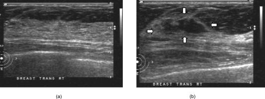

Fig. 9

Results of fitted background optical properties versus iteration numbers. (a) and (c) Fitted optical absorption coefficient versus iteration for first and second layers, respectively, and (b) and (d) fitted reduced scattering coefficient versus iteration for first and second layers, respectively. The fitting algorithm converges around iteration number 226.

Fig. 10

(a) to (c) Reconstructed optical absorption maps at (a) $780\mathrm{nm}$ and (b) $830\mathrm{nm}$ and the computed total hemoglobin map (c) using semi-infinite model. Reconstructed absorption coefficients were $0.121{\mathrm{cm}}^{-1}$ $\left(780\mathrm{nm}\right)$ , $0.124{\mathrm{cm}}^{-1}$ $\left(830\mathrm{nm}\right)$ , and $57.69\mu \mathrm{mol}∕\mathrm{l}$ (total hemoglobin). (d) to (f) Reconstructed optical absorption maps at (d) $780\mathrm{nm}$ and (e) $830\mathrm{nm}$ and the computed total hemoglobin map (f) using the layer-based model. Reconstructed absorption coefficients were $0.0832{\mathrm{cm}}^{-1}$ $\left(780\mathrm{nm}\right)$ , $0.113{\mathrm{cm}}^{-1}$ $\left(830\mathrm{nm}\right)$ , and $47.09\mu \mathrm{mol}∕\mathrm{l}$ (total hemoglobin). In each figure, the first slice is the spatial $x\text{-}y$ image $0.5\mathrm{cm}$ deep from the skin surface and the last slice is $3.0\mathrm{cm}$ toward the chest wall. The dimension of each slice is $9\times 9\mathrm{cm}$ and the spacing between the slices is $0.5\mathrm{cm}$ . The vertical scale is absorption coefficient in inverse centimeters or total hemoglobin concentration in micromoles per liter.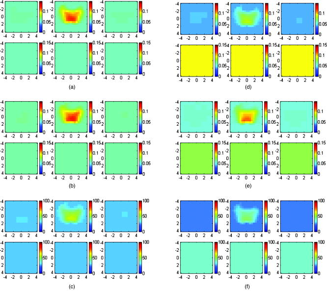

Figure 11 shows the ultrasound images obtained from the contralateral and lesion sites of a $61\text{-}\text{year}$ -old patient. It can be seen from Fig. 11a that the lesion is about $1.2\mathrm{cm}$ deep and the breast tissue and chest-wall layer interface is almost flat with a breast layer thickness of about $1.4\text{to}1.5\mathrm{cm}$ . The fitted background optical properties of the breast and chest-wall tissue obtained from the contralateral normal breast were ${\mu }_{a1}=0.079{\mathrm{cm}}^{-1}$ , ${\mu }_{s1}^{\prime }=4.21{\mathrm{cm}}^{-1}$ , ${\mu }_{a2}=0.086{\mathrm{cm}}^{-1}$ , and ${\mu }_{s2}^{\prime }=5.93{\mathrm{cm}}^{-1}$ at $780\mathrm{nm}$ , and ${\mu }_{a1}=0.088{\mathrm{cm}}^{-1}$ , ${\mu }_{s1}^{\prime }=4.38{\mathrm{cm}}^{-1}$ , ${\mu }_{a2}=0.11{\mathrm{cm}}^{-1}$ , and ${\mu }_{s2}^{\prime }=6.76{\mathrm{cm}}^{-1}$ at $830\mathrm{nm}$ . The fitted optical properties by using the semi-infinite method directly were ${\mu }_a=0.079{\mathrm{cm}}^{-1}$ , and ${\mu }_s^{\prime }=4.29{\mathrm{cm}}^{-1}$ at $780\mathrm{nm}$ and ${\mu }_a=0.091{\mathrm{cm}}^{-1}$ and ${\mu }_s^{\prime }=4.38{\mathrm{cm}}^{-1}$ at $830\mathrm{nm}$ . The absorption maps and the computed total hemoglobin map obtained from with the semi-infinite approximation are shown in Figs. 12a, 12b, 12c and those from the two-layer model are shown in Figs. 12d, 12e, 12f. Both images show high absorption and therefore high total hemoglobin concentration with layer-based reconstruction providing higher values. Ultrasound-guided core biopsy confirmed that the lesion was an early stage invasive carcinoma with ductal and lobular features. These examples demonstrate that the layer-based imaging reconstruction has a great potential to improve the contrast between malignant and benign lesions and therefore provide more accurate diagnosis.

Fig. 11

Ultrasound images obtained from a $61\text{-}\text{year}$ -old patient who has a suspicious mass: (a) contralateral normal site and (b) lesion site.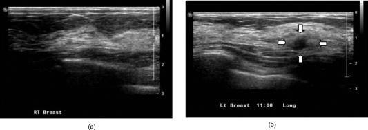

Fig. 12

(a) to (c) Reconstructed optical absorption maps at (a) 780 and (b) $830\mathrm{nm}$ and the computed total hemoglobin map (c) using the semi-infinite model. Reconstructed absorption coefficients were $0.232{\mathrm{cm}}^{-1}$ $\left(780\mathrm{nm}\right)$ , $0.238{\mathrm{cm}}^{-1}$ $\left(830\mathrm{nm}\right)$ , and $111.33\mu \mathrm{mol}∕\text{liter}$ (total hemoglobin). (d) to (f) Reconstructed optical absorption maps at (d) 780 and (e) $830\mathrm{nm}$ and the computed total hemoglobin map (f) using the layer-based model. Reconstructed absorption coefficients were $0.247{\mathrm{cm}}^{-1}$ $\left(780\mathrm{nm}\right)$ , $0.293{\mathrm{cm}}^{-1}$ $\left(830\mathrm{nm}\right)$ , and $126.39\mu \mathrm{mol}∕\text{liter}$ (total hemoglobin). In each figure, the first slice is the spatial $x\text{-}y$ image of $0.2\text{-}\mathrm{cm}$ depth from the skin surface and the last slice is $3.0\mathrm{cm}$ toward the chest wall. The dimensions of each slice are $9\times 9$ cm and the spacing between the slices is $0.5\mathrm{cm}$ . The vertical scale is absorption coefficient in inverse centimeters or total hemoglobin in the unit of micromoles per liter.