|
|
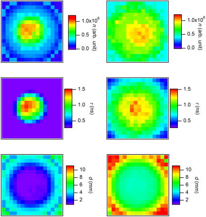
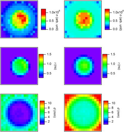
1.IntroductionCancer is a major public health problem worldwide. Currently, one in four deaths in the United States is caused by cancer.1 Breast cancer has been one of the dominant causes for the deaths of women in the United States.1 Since breast cancer is spread easily by metastasis, its early detection is crucial. Systematic use of x-ray mammography has been extremely beneficial in detecting breast cancer and is the gold standard. However, the potential risk related with repetitive exposure to this ionizing radiation technique2 has led to the development of complementary diagnostic methods using nonionizing techniques such as near-infrared (NIR)optical imaging.3, 4 Optical fluorescence molecular imaging has the potential to provide clinical information in biomedical applications such as tissue oxygenation, glucose levels, and small molecule protein-protein interactions5 as well as the early detection of cancer. There are two main approaches to optical fluorescence molecular imaging in a tissue-like turbid medium: continuous-wave (cw)intensity measurement and time-domain (TD) measurement (or its frequency domain equivalent), where the fluorescence temporal response (order of nanoseconds) to a short pulse (order of picoseconds) of excitation light is recorded and known as a fluorescence temporal point-spread function (TPSF). The cw technique is most widely used due to its simple and inexpensive implementation. However, unlike the cw technique that typically provides 2-D images of fluorescent cw intensity, the TD technique has the opportunity to further provide the concentration , lifetime , and depth of a fluorescent inclusion. cw tomographic methods have been adopted to try and solve the problem of decoupling fluorescence intensity into and , where multiple source-detector pair cw measurements are acquired at many angles with complicated and intensive inversion processes.6 Alternatively, only one source-detector pair measurement is needed to recover and with a TD technique, as previously published.7 More recently,8 we described a simple method for recovering and of a fluorescent inclusion from direct evaluations of the temporal position of the fluorescence temporal point-spread function (TPSF) maximum and the exponential time decay of a given fluorescence TPSF, so-called effective lifetime . Here, we simultaneously evaluate all three parameters, i.e., , , and of a fluorescent inclusion, by fitting the complete fluorescence TPSF with an analytical diffusion model of photon propagation. 2.Theory2.1.Photon Migration in a Turbid MediumUltimately, the best way to provide a thorough description of a photon migration in a turbid medium is TD diffuse optical tomography, which decouples the underlying scattering and absorption of photons. NIR photon migration in a turbid medium is governed by the diffusion equation for the diffuse photon fluence rate , where is the speed of light in the medium, is the optical absorption coefficient, is the optical scattering coefficient, is the mean cosine of the scattering angle, is the photon source at a source location , is the diffusion coefficient, and is the reduced scattering coefficient. is usually approximated to be , since scattering is dominant over absorption in a turbid medium. For a short pulse from an isotropic point source, if we assume that and are position independent, i.e., and , then the solution to Eq. 1 becomes Green’s function.9, 10 which describes the light propagation in a turbid medium.2.2.Light Propagation ModelA schematic diagram of the experimental setup of the eXplore Optix™-MX2 system (ART Advanced Research Technologies, Inc., Montreal, Canada) is shown in Fig. 1c . As shown in Fig. 1c, the whole light propagation procedure from source to detector can be divided into four steps: Green’s function representing a photon migration from source to a fluorescent inclusion , lifetime decay of a fluorescent inclusion, another Green’s function showing a migration from a fluorescent inclusion to detector , and impulse response function (IRF) of approximated Gaussian wave form. In general, and are functions of wavelength, thus the steps and should be described by different propagators. However, since the excitation and emission wavelength are close to each other where tissue optical properties vary slowly, these Green’s functions can be described by the same propagator. A summary of the previous procedure can be written as the forms of the following analytical functions, where is a lifetime of a fluorescent inclusion and represents the central temporal position of the Gaussian IRF with a width of . Under this formulation, the use of the standard first-order Born approximation11, 12 gives us a resulting reflective fluorescence fluence rate at a detector position from a fluorophore distributed in a volume ,where is a constant including source/detector efficiencies and a filter loss. Here represents the product of the concentration and its quantum efficiency (which is known a priori), and ∗ denotes the convolution.Fig. 1(a) Reflection geometry is composed of a single source-detector pair ( separation), which is raster scanned every across the phantom surface ( area) encompassing the submerged fluorescent inclusion. (b) Side view of (a). (c) Schematic diagram of the experimental setup for the propagator description of photon migration.  To generate a fluorescent distribution in the region of interest, the integral in Eq. 4 is to be discretized [ , , , , , , , , ]. For a series of measurements that have been made at source and detector positions, Eq. 4 turns to the following matrix equation, 3.Materials and Methods3.1.The eXplore Optix™-MX2 SystemThe eXplore Optix™-MX2 system is the only commercially available multiwavelength (470, 635, 670, and ) TD optical molecular imaging system for small animals.13 The laser pulse width was approximately and the temporal resolution of the detection system was approximately . Schematic scanning geometry is depicted in Figs. 1a and 1b. Scanning resolution was per step over the region of interest (ROI) with a scan time of per step. The ROI was a square of area within which a small cylindrical Cy5 or Cy7 inclusion was submerged in the optical scattering Intralipid medium. The system uses a single source-detector configuration to scan the small animal in reflection mode, and measures the fluorescence TPSF for each scanned pixel. The fluorescence TPSFs were used to quantify , , and of the fluorescent inclusion. 3.2.Phantom ManufactureTo expedite repeated and robust experiments, we manufactured solid optically scattering fluorescent pellets with either Cy5 or Cy7 at , similar to a method that is found in the literature.14 The diameter and the height of these cylindrical pellets were 15 and , respectively. 4.Results and Discussion4.1.Temporal Evolution of the Light PropagationIn the forward problem we use Eq. 4 to model the light propagation and resulting fluorescence TPSF given a priori optical properties of a turbid medium and the fluorophore inclusion properties. Figure 2 shows the evolution of the fluorescence TPSF at each propagation step with normalized maximum intensity to highlight the increasing temporal convolution form. To validate the forward model, we used the optical properties from the phantom experiment with a Cy5 fluorophore inclusion (i.e., , , , and ). Rather than attempting to calibrate the experiment intensity units to model intensity units, we simply display the normalized maximum intensity experimental data in Fig. 2 and demonstrate that the forward model can predict the correct shape of the experimental fluorescence TPSF. Moreover, since the model assumes a point fluorophore and experimentally we have a finite fluorescent inclusion, it is not strictly possible to model the absolute fluorophore concentration, although we can still compare fluorophore concentration in arbitrary units within this point-model approximation. From Fig. 2 it can also be seen that the time decay of the fluorescence TPSF is largely dominated by the lifetime decay of the fluorescent inclusion. However, the so-called effective lifetime indicating the time decay of a fluorescence TPSF is not the same as the actual lifetime of a fluorescent inclusion due to the convolution of its lifetime decay with two Green’s functions and the IRF. For more detailed analysis, the increase in the decay of the fluorescence TPSF is evaluated by fitting it with a monoexponential function from 80% peak intensity to 20% peak intensity as the photons propagate from source to detector. The first Green’s function , i.e., the propagation of light from source to a fluorescent inclusion in a turbid medium, shows a rapid decay of only , which does not contribute significantly to the effective lifetime of the resultant fluorescence TPSF, which is . After photons excite the fluorescent inclusion to cause fluorescence emission, the decay of the consequent function is , which is a significant component of the effective lifetime. When convoluted with another Green’s function , there is a slight increase in the decay of the consequent function to . Finally, convolution with the system IRF adds further increase, resulting in the fluorescence TPSF , whose decay is and is the effective lifetime. 4.2.Effect of Background Optical Properties on the Fluorescence Temporal Point-Spread FunctionWe assumed the background optical properties were known accurately a priori. However, in vivo we have to estimate the optical properties of the mouse where inaccuracy can introduce error in recovering , , and of the fluorophore. To mimic this condition, we used the forward model to generate fluorescence TPSFs for a variety of background optical properties (5% change in or from initial values). We then fitted these fluorescence TPSFs with the model fixing the background optical properties to the initial values and investigated the impact on the recovered fitted values of , , and . We found that there was negligible error in and (0.5%). Interestingly, Fig. 3 shows the fluorescence TPSFs normalized to maximum intensity, where it is observed that the temporal shape of the fluorescence TPSF for the different values of [Fig. 3a] and [Fig. 3b] is similar. Since previous work8 has shown that and are strongly correlated with the temporal shape of the fluorescence TPSF, i.e., and , it is expected that similar and values were recovered. However, varying the background optical properties also influences the absolute area of the fluorescence TPSF, which was found to induce a 10% error in that essentially scales the intensity signal without changing the temporal shape. Nevertheless, recovery of fluorophore concentration within 10% would still be a useful result, given that the background optical properties can be estimated a priori within 5%. 4.3.Phantom AnalysisIn this section we analyze experimental phantom data from Cy5 and Cy7 fluorescent inclusions submerged in a turbid medium. The background optical properties of the phantom were as follows: , at (for Cy5), and , and at (for Cy7).15 The eXplore-Optix-MX2 scanned the phantom and acquired fluorescence TPSFs as described before. Model fitting involved first averaging the fluorescence TPSFs from a region of interest covering the fluorescent pellet to extract an average value of , , and with a priori background optical properties. Using the average values as an initial guess, we then fitted the model [Eq. 5] on a pixel-by-pixel basis. The difference between the measured and calculated fluorescence TPSF in each pixel was minimized using a least-squares nonlinear optimization routine, i.e., the Levenberg-Marquardt algorithm.16, 17 For example, Fig. 4 shows a final fit result for a given pixel from the Cy5 fluorescent inclusion after 88 iterations from initial average parameters with a priori knowledge of the background optical properties ( and ), as well as , and at . Recovered fitted values of , , and were obtained. Fig. 4Example fit result from Cy5 inclusion using the algorithm described in Eq. 5 with a priori values of , , , and at . Recovered fit values are evaluated as , , and .  Displaying the recovered fitted values of , , and for each scanned pixel generated corresponding 2-D images of these parameters. Since the model assumes a point fluorophore at depth directly below the surface, we recover appropriate values for the inclusion as we scan across it. However, as we scan away from the inclusion, the model breaks down and we no longer recover appropriate values. In essence, the model corrects for optical propagation in the axis but not in the scanning plane where optical scattering increases the apparent size of the inclusion. Figure 5 show images of (top row), and (bottom row) of the Cy5 fluorescent inclusion submerged at (left) and (right), respectively. Figure 6 shows the corresponding images for the Cy 7 fluorescent inclusion. In Fig. 5 (top), it is seen in the vicinity of the inclusion that similar values of are recovered at 1- and submersion as expected, since the fluorophore concentration remained constant, even though the cw intensity diminished with increasing depth. In Fig. 5 (middle), it is seen in the vicinity of the inclusion that similar values of are recovered at 1- and submersion as expected, since the fluorophore lifetime remained constant even though the effective lifetime increased with increasing depth. In Fig. 5 (bottom), it is seen in the vicinity of the inclusion that different values of ( and ) are recovered at 1- and submersion as expected, since the fluorophore depth increased. Note the submersion depth is defined as the perpendicular distance to the top surface of the fluorescent inclusion. Given that we have a point model and a finite inclusion, it is expected to slightly overestimate , as discussed elsewhere.8 Similar results were found for the Cy 7 fluorescent inclusion as seen in Fig. 6, where fitted values of , , and ( and ) were recovered. 5.ConclusionA time-domain optical method to evaluate the concentration, lifetime, and depth of a fluorescent inclusion is described by the complete analysis of the fluorescence temporal point-spread function (TPSF). The sensitivity of these parameters to a priori estimates of background optical properties is explored. We demonstrate the approach by fitting the model to experimental data from a localized fluorescent inclusion in scattering media. 2-D images of , , and parameters are created from either Cy5 and Cy7 fluorescent inclusions submerged at depths of 1 or . The model is able to recover the correct submersion depths, which also yield similar fluorophore concentrations and similar correct lifetimes as expected. Optical scattering still blurs the images in the plane, and we plan to address this in future work. The method has potential applicability for in vivo fluorescence imaging where the point model is found to be adequate, i.e., localized fluorescent tumors. AcknowledgmentsThe authors gratefully acknowledge the UCSD Department of Radiology and the NIH (grant No. S10 RR22599-01A1) for funding this work. ReferencesA. Jemal,
R. Siegel,
E. Ward,
T. Murray,
J. Xu, and
M. J. Thun,
“Cancer statistics, 2007,”
Ca-Cancer J. Clin., 57 43
–66
(2007). 0007-9235 Google Scholar
“1990 recommendations of the International Commission on Radiological Protection,”
ICRP Publication 60,
(1991) Google Scholar
V. Ntziachristos,
J. Ripoll,
L. V. Wang, and
R. J. Weissleder,
“Looking and listening to light: the evolution of whole-body photonic imaging,”
Nat. Biotechnol., 23 313
–320
(2005). https://doi.org/10.1038/nbt1074 1087-0156 Google Scholar
R. Weissleder and
V. Ntziachristos,
“Shedding light onto live molecular targets,”
Nat. Methods, 9 123
–128
(2003). 1548-7091 Google Scholar
T. H. Pham,
F. Bevilacqua,
T. Spott,
J. S. Dam,
B. J. Tromberg, and
S. Anderson-Engels,
“Quantifying the absorption and reduced scattering coefficients of tissue-like turbid media over a broad spectral range with non-contact Fourier-transform hyperspectral imaging,”
Appl. Opt., 39 6487
–6497
(2000). 0003-6935 Google Scholar
E. E. Graves,
J. Ripoll,
R. Weissleder and
V. Ntziachristos,
“A submillimeter resolution fluorescence molecular imaging system for small animal imaging,”
Med. Phys., 30 901
–911
(2003). https://doi.org/10.1118/1.1568977 0094-2405 Google Scholar
D. Hall,
G. Ma,
F. Lesage, and
Y. Wang,
“Simple time-domain optical method for estimating the depth and concentration of a fluorescent inclusion in a turbid medium,”
Opt. Lett., 29 2258
–2260
(2004). https://doi.org/10.1364/OL.29.002258 0146-9592 Google Scholar
S. H. Han and
D. J. Hall,
“Estimating the depth and lifetime of a fluorescent inclusion in a turbid medium using a simple time-domain optical method,”
Opt. Lett., 33
(9), 1035
–1037
(2008). https://doi.org/10.1364/OL.33.001035 0146-9592 Google Scholar
S. Chandrasekhar,
“Stochastic problems in physics and astronomy,”
Rev. Mod. Phys., 15 1
–89
(1943). https://doi.org/10.1103/RevModPhys.15.1 0034-6861 Google Scholar
M. S. Patterson,
B. Chance, and
B. C. Wilson,
“Time resolved reflectance and transmittance for the noninvasive measurement of tissue optical properties,”
Appl. Opt., 28 2331
–2336
(1989). 0003-6935 Google Scholar
M. A. O’Leary,
D. A. Boas,
X. D. Li,
B. Chance, and
A. G. Yodh,
“Fluorescence lifetime imaging in turbid media,”
Opt. Lett., 21 158
–160
(1996). https://doi.org/10.1038/021158a0 0146-9592 Google Scholar
V. Ntziachristos and
R. Weissleder,
“Experimental three-dimensional fluorescence reconstruction of diffuse media by use of a normalized Born approximation,”
Opt. Lett., 26 893
–895
(2001). https://doi.org/10.1364/OL.26.000893 0146-9592 Google Scholar
D. Hall and
S. H. Han,
“Preliminary results from a Multi-wavelength time domain optical molecular imaging system,”
Proc. SPIE, 6430 64300T
(2007). 0277-786X Google Scholar
M. Firbank,
M. Oda, and
D. T. Deply,
“An improved design for a stable and reproducible phantom material for use in near-infrared spectroscopy and imaging,”
Phys. Med. Biol., 40 955
–961
(1995). https://doi.org/10.1088/0031-9155/40/5/016 0031-9155 Google Scholar
H. J. van Staveren,
C. J. M. Moes,
J. van Marle,
S. A. Prahl, and
M. J. C. van Gemert,
“Light scattering in Intralipid-10% in the wavelength range of ,”
Appl. Opt., 30 4507
–4514
(1991). 0003-6935 Google Scholar
K. Levenberg,
“A method for the solution of certain non-linear problems in least squares,”
Q. Appl. Math., 2
(2), 164
–168
(1944). 0033-569X Google Scholar
D. W. Marquardt,
“An algorithm for least-squares estimation of nonlinear parameters,”
Soc. Indust. Appl. Math., 11
(2), 431
–441
(1963). Google Scholar
|