Compact portable ocular microtremor sensor: design, development and calibration

James Patrick Ryle; Mohammed Ali Al-Kalbani; Niamh Collins; Unnikrishnan Gopinathan; Gerard Boyle; Davis Coakley; John T. Sheridan

doi:10.1117/1.3083435

1 January 2009 Compact portable ocular microtremor sensor: design, development and calibration

James Patrick Ryle, Mohammed Ali Al-Kalbani, Niamh Collins, Unnikrishnan Gopinathan, Gerard Boyle, Davis Coakley, John T. Sheridan

Author Affiliations +

Journal of Biomedical Optics, Vol. 14, Issue 1, 014021 (January 2009). https://doi.org/10.1117/1.3083435

Abstract

Ocular microtremor (OMT) is a physiological high-frequency (up to 150 Hz) low-amplitude (25–2500 nm peak-to-peak) involuntary motion of the human eye. Recent studies suggest a number of clinical applications for OMT that include monitoring the depth of anesthesia of a patient in surgery, prediction of outcome in coma, and diagnosis of brain stem death. Clinical OMT investigations to date have used mechanical piezoelectric probes or piezoelectric strain gauges that have many drawbacks which arise from the fact that the probe is in contact with the eye. We describe the design of a compact noncontact sensing device to measure OMT that addresses some of the above drawbacks. We evaluate the system performance using a calibrated piezoelectric vibrator that simulates OMT signals under conditions that can occur in practice, i.e., wet eye conditions. We also test the device at low light levels well within the eye safety range.

1. Introduction

Ocular microtremor (OMT) is a fine involuntary tremor of the eye caused by constant activity of the brainstem oculomotor units.¹ Along with drift and microsaccades, it is one of the three fixational eye movements described by Alder and Fliegelman in 1934.² Since then the existence of OMT in humans has been confirmed by many authors,^{1, 3, 4, 5, 6, 7, 8, 9, 10} and OMT observations have also been made on cats,¹¹ rabbits,¹² and rats.¹³

Accurate OMT measurement could prove a useful tool to aid clinical diagnosis of a number of conditions. Previous investigations using contact methods have looked at OMT as a method of unambiguous brain stem death confirmation,¹⁴ prediction of the outcome of coma,¹⁵ monitoring patients depth of anaesthesia,^{16, 17, 18} and atypical OMT records have been observed in patients with Parkinson’s disease¹⁹ and multiple sclerosis.²⁰ A decrease in peak OMT frequency with age, of clinically normal patients, has also been documented.²¹ In addition to this, the role of OMT and the other fixational eye movements on the visual process have also been suggested.²²

Eye motion amplitudes are customarily quoted in the literature in units of angular rotation of the eye. During the system development, calibration, and testing it has been more convenient to express displacement (obtained from the change in phase of the optical beam) in terms of linear rather than angular units (i.e., meters as opposed to arcsec). We note, however, that a $1 arcsec$ rotation corresponds to a $56 nm$ displacement for a typical eye of diameter of $23 mm$ . OMT has a random, noiselike appearance with intermittent sinusoidal bursts. The peak-to-peak (pk-pk) amplitude of OMT is of the order of $1 μ m$ $(17.86 arcsec)$ , with an estimated range from $150 to 2500 nm$ (pk-pk) $(2.67 to 44.64 arcsec)$ . However, to accurately observe OMT, a minimum resolution of $25 nm$ (pk-pk) $(0.45 arcsec)$ has been suggested to be necessary.¹⁰ OMT in clinically normal humans has a frequency range from $40 to 100 Hz$ , peaking at around $88 Hz$ . However, frequency observations between 10 and $150 Hz$ have been made.¹⁰ As the frequency range of OMT is much greater than drift or microsaccades, OMT is considered a physiological high-frequency signal relative to the other fixational eye movements.

Far field methods have been used to observe OMT,⁷ however, we are aware of only one other that has used a speckle-based technique.^{10, 23} Previous noncontact-based studies have observed the minute motion of OMT using contact lenses placed on the eye. However, such methods, involving the use of a contact lens embedded with either a mirror or an embedded search coil, are impractical and too invasive for a clinical situation. However, by using the resulting reflected light beam which deflected proportionally to the eye movement, investigators were able to detect OMT.^{2, 3, 5} When exposed to an ac magnetic field, the current induced in an embedded search coil can be used to determine the orientation of the eye relative to the field. In the 1950s, researchers were able to determine the amplitude and frequency of OMT optically⁷ using a blood vessel in the eye as a reference point, with a slit camera used to take photographs at a constant velocity. Far-field, noncontact, optically based convolution methods are attractive for their apparent simplicity and ease of use, however, the cost and the relatively low sampling rates of multipixel digital cameras have to date hindered their application in the measurement of OMT.

A number of studies observing OMT using the mechanical contact probe method have been performed.^{4, 8, 16, 17, 19} A length of piezoelectric material, covered by a protective covering of silicone, makes contact with the eye by means of a sprung screw mechanism. Despite resolution as low as $10 nm$ (pk-pk), a number of drawbacks exist with this method. It does not give accurate information about the amplitude of the movement, as the voltage is proportional to the degree of contact made between the piezoelectric material and the eye. Also, by mechanically loading the eye, this method may significantly dampen the eye’s movement. While this is useful in filtering out large movements such as drift, it affects the measured OMT results as well. In addition, the eye must be anaesthetized, which induces blepharospasm, spasm of the eyelid in some patients. Apart from being highly uncomfortable to the patient, the contact method requires the use of sterile piezoelectric probes for each examination, increasing the difficulty and cost.

In the late 1990s, Boyle²³ designed and built a speckle interferometer using bulk optics clamped to a large optical bench to measure OMT. An optical beam originating from a HeNe laser was split using a half-mirror beamsplitter with phase modulation of the reference beam in the interferometer achieved through mechanical vibration of a mirror positioned in one arm of the interferometer. This system required subjects to focus at a point while clinicians took readings. The physical bulk of the system reduced the probability of its invivo applications. Furthermore, the minimum displacement resolution achieved using this system was $100 nm$ (pk-pk). This is 4 times greater than the suggested minimum sensitivity for accurate resolution of the OMT.¹⁰

Speckle interferometric techniques have advanced significantly since the work carried out by Leendertz in the late 1960s and early 1970s.²⁴ Laboratory heterodyne speckle interferometric systems, for example, have been demonstrated to be capable of measuring microvibrations with amplitudes down to $1 nm$ . However, in that case the lowest frequency measured was $5 kHz$ with a laser output power of $2 mW$ . For a device capable of measuring OMT, the system must, as stated, be able to measure microvibrations with amplitudes from $150 to 2500 nm$ (pk-pk) and a frequency range of $10 - 150 Hz$ at low laser output power levels, i.e., at intensity values which will not cause retinal damage.

This paper is structured as follows. In Sec. 2 we first present some theory concerning in-plane displacement measurement using speckle interferometry. A rough surface is illuminated by two coherent beams, and after experiencing in-plane motion, the phase of one beam increases while the other decreases. Estimating the relative phase change by measuring the resulting intensity changes in the interference of the two beams enables us to determine the magnitude of the microvibrations The design of a compact noncontact OMT sensing device is described in Sec. 3, We also comment on the safe optical power levels with regard to accidental retinal exposure to laser radiation. In order to make the device portable, the optical components are coupled together using optical fibers. A lithium niobate crystal is used to split the optical beam output by the laser diode and also to modulate the relative phase of the beams. Thus, the size of the system is reduced, enabling greater portability with a view to realizing a compact diagnostic tool for use in clinical settings. In Sec. 4 we describe the performance and evaluate the device using an OMT simulator under conditions that simulate a wet eye surface. The device is also tested at low light levels that fall well within safe levels for the human eye. Finally, in Sec. 5 we present a discussion of the test results and the practical issues that need to be addressed for the device to be used as a practical tool for in-vivo use by clinicians.

2. Principle of Operation

Leendertz proposed a two-beam illumination method to detect in-plane displacement in one component of the direction using the speckle effect. An area of the target surface is symmetrically illuminated by two mutually coherent beams incident at equal angles, $α$ , to the surface normal. The image at the observation plane, $P (x, y)$ , in Fig. 1 is normal to the point of intersection of the two beams. It consists of two independent, coherent speckle patterns arising due to each beam. A change in the relative phase of the two patterns gives rise to an intensity variation proportional to the in-plane surface distance moved.

Fig. 1

Schematic showing Leendertz’s method to measure motion using the speckle effect showing propagation vectors, and two collimating laser beams interfering at angles $α$ to the normal.

The electromagnetic propagation vector of the illuminating beams in Fig. 1 is defined as

Eq. 1

k_{m} = \frac{2 π}{λ} n_{m},

with

m = {1, 2}

for each illuminating beam,

n_{m}

are the unit vectors in the direction of illumination beam propagation, and

λ

is the wavelength of the source. The change of the observed phase

φ_{0}

at the

P (x, y)

is caused by a relative in-plane displacement of the surface described by the vector

L

,

Eq. 2

φ_{0} = k \cdot L,

where

k

is the propagation vector in the observed direction, and the “⋅” indicates a vector dot product. The phase change accumulated by each beam in propagating this distance is given by

Eq. 3

φ_{m} = k_{m} \cdot L,

with once again

m = {1, 2}

for each illuminating beam. The resultant phase shift between speckle points at the observation plane is

Eq. 4

φ_{d} = (φ_{0} - φ_{1}) - (φ_{0} - φ_{2}) .

By replacing each path phase in Eq. 4 with the path phases from Eqs. 2, 3, the resultant phase shift in the plane

P (x, y)

due to the displacement vector

L

of the rough surface is given by

Eq. 5

φ_{d} = (k_{2} - k_{1}) \cdot L .

However, with the beams extending in the

X Y

plane at equal angles “

α

” to the normal, with vectors

i

,

j

, and

k

lying in the

X

,

Y

, and

Z

planes as shown in Fig. 1, this reduces to

Eq. 6

φ_{d} = \frac{2 π}{λ} {[\sin (α) j + \cos (α) k] - [- \sin (α) j + \cos (α) k]} \cdot L = \frac{2 π}{λ} 2 \sin (α) j \cdot L .

Thus, the only component of motion for this method of illumination is in the

j

direction, and a displacement vector of magnitude

d

and direction along the vector

j

results in the following phase change,

Eq. 7

φ_{d} = \frac{4 π}{λ} \sin (α) d .

This is also true for in-plane time-varying displacement

d (t)

. Baseband displacement information can be shifted up the frequency spectrum in order to eliminate unwanted low-frequency optical signals introduced, for example, by the ambient room lighting. This is achieved by modulating one beam’s phase relative to the other. Assuming point detection by a photodiode, and that a sufficient number of speckles (i.e.,

\sim 100

) always populates the photosensitive area of the photodiode, thus keeping the average optical power constant, the modulated interference signal will take the form

Eq. 8

s (t) = U_{0} \cos [β \cos (ω_{c} t) + φ_{d} + ψ_{0}],

where

U_{0}

and

ψ_{0}

are random amplitude and phase components.²⁵ Modulation depth is denoted by

β

, and

ω_{c} = 2 π f_{c}

is the angular frequency of the carrier frequency

f_{c}

. For very small movement, we can assume

U_{0} = 1

and

ψ_{0} = 0

. By expanding Eq. 8 using the Bessel²⁶ series we get

Eq. 9

s (t) = \cos [\frac{4 π}{λ} \sin (α) d (t)] [J_{0} (β) - 2 J_{2} (β) \cos (2 ω_{c} t) + 2 J_{4} (β) \cos (4 ω_{c} t) \dots] - \sin [\frac{4 π}{λ} \sin (α) d (t)] [2 J_{1} (β) \cos (ω_{c} t) - 2 J_{3} (β) \cos (3 ω_{c} t) + \dots],

where

J_{n} (β)

is a Bessel function of the first kind. In order to separate the movement signal from the phase-modulated signal, phase demodulation is necessary. In-quadrature signals are obtained by performing synchronous demodulation at the carrier frequency

ω_{c}

, and at the first harmonic of the carrier frequency at

2 ω_{c}

, this yields

10.

s_{s} (t) = 2 J_{1} (β) \sin [\frac{4 π}{λ} \sin (α) d (t)], and

s_{c} (t) = 2 J_{2} (β) \cos [\frac{4 π}{λ} \sin (α) d (t)] .

By controlling the modulation depth

β

, it is possible to set

J_{1} (β) = J_{2} (β)

. In this case, taking the arctangent of the ratio of

s_{s} (t)

to

s_{c} (t)

gives

Eq. 11

ϕ_{w} (t) = \arctan [\frac{s_{s} (t)}{s_{c} (t)}],

where

ϕ_{w} (t)

is the wrapped phase information related to the in-plane movement. The arctangent function is bound to the range [

- π ∕ 2

,

π ∕ 2

] radians, and as a result the phase of the motion is discontinuous and phase wrapped, where we recall that

π

corresponds to one half of a phase cycle of the optical wavelength used. Phase unwrapping is the process whereby integer multiples of

π

are added or subtracted to the wrapped signal to achieve a continuous phase signal,

ϕ_{d} (t)

. Applying this process, the amplitude is found by converting the unwrapped phase signal into distance using known system parameter values,

Eq. 12

d (t) = \frac{1}{\sin (α)} \frac{λ}{4 π} ϕ_{d} (t) .

Assuming shot noise limited detection, the maximum signal-to-noise ratio (SNR) is^{25, 27}

Eq. 13a

SNR = \frac{I_{s} η}{2 h ν B},

where

I_{s} = T I_{l} λ^{2} ∕ π D^{2}

, and the minimum amplitude that can be measured (sensitivity) is then given by

Eq. 13b

{(d_{0})}_{\min} = \frac{λ}{2 π \sin (α)} \frac{1}{\sqrt{SNR}} .

In Eq. 13a,

I_{s}

represents the optical power in one laser speckle,

η

is the quantum efficiency of the detector,

h ν

is the photon energy, and

B

is the bandwidth (Hz) of the system.

T

is the transmission factor of the optical system and allows for losses, including diffuse reflection at the rough surface,

I_{L}

is the laser output power, and

D

is the diameter of the illuminating light spot on the surface. Clearly the illuminating spot size has a bearing on the sensitivity of the system and should be kept to a minimum. Similarly, the laser power

I_{L}

should be large enough to give the required sensitivity without posing a danger to the patient.

3. Design and Development of a Noncontact OMT Sensor

In designing a noncontact optical system to measure OMT, the safety of the subjects’ eyes is paramount. This optical noncontact system is designed so only a small area on the sclera, i.e., the white of the eye, is illuminated with laser radiation, and thus fixational eye movements, in particular OMT, are recorded using light scattered from the sclera alone. It is not intended that any laser light enter the pupil itself.

3.1.

Laser Safety Standards

The principle contributors to retinal damage are due to effects from thermal, thermoacoustic, and photochemical interactions between internal eye tissue and the laser radiation.²⁸ Safety standards²⁹ exist to protect the human eye from retinal damage due to exposure from laser radiation. In our systems, to measure fixational eye movements, only scleral illumination with laser radiation is necessary. However, for nonintentional exposure to laser light of wavelengths in the range $400 - 700 nm$ , for time periods of between $10 s$ and $5 \min$ , the maximum permissible exposure limit (MPE), in Joules per meter squared $(J m^{- 2})$ , is calculated using the following equation:

Eq. 14

MPE = {\begin{cases} 10^{2} C_{3} C_{6} \\ 18 t^{0.75} C_{6} \end{cases} if \begin{array}{l} t > T_{2} \\ t < T_{2} \end{array} .

C_{3}

is a wavelength-dependant correction factor, and

C_{6}

is a correction factor dependant on the visual angle with which the laser radiation enters the pupil. The exposure duration is denoted by

t

. For direct viewing of the laser radiation²³ (i.e., small visual angles),

C_{6} = 1

.

T_{2}

, the exposure duration limit, is given by

Eq. 15

T_{2} = 10 \times 10^{0.02 (g - 550)},

where

g = λ \times 10^{9}

. Therefore for a

638 nm

source,

T_{2} = 575 s

. Because we are only interested in short exposures, i.e.,

t < T_{2}

, this is the expression used to calculate the MPE later in this paper. Therefore, the MPE, in Watts per meter squared

(W m^{- 2})

, is

MPE = 18 t^{- 0.25} C_{6}

. Assuming direct “intrabeam” accidental direct exposure of the retina

(C_{6} = 1)

and a pupil close to full dilation with a diameter of

7 mm

, the light intensity is averaged over this area

(38.48 \times 10^{- 6} m^{2})

. Thus the expression for the MPE limit in Watts (W) becomes

Eq. 16

MPE = 6.927 \times 10^{- 4} t^{- 0.25} .

This expression is derived from the International Electrotechnical Commission’s 1993 (IEC 825-1) safety standards.²⁹ We note, however, that Delori’s recent paper²⁸ reviewed the American National Standards Institute’s (ANSI Z136.1-2000) safety standards. For accidental retinal exposures

(t < 0.7 s)

, the pupil function in Ref. 28 becomes unity, resulting in an equivalent expression for the MPE limit presented here. These results can be applied to our system in order to determine the permissible exposure time for the laser power used.

3.2.

Compact Optical System Design

The main components in our system, as seen in Fig. 2, include (i) laser diode source, (ii) $Y$ -junction phase modulator, (iii) interconnecting optical fibers, (iv) collimating lenses, (v) photodetector and amplifier, and (vi) an analog to digital converter. Postcapture phase unwrapping, and displacement signal extraction is then performed.

Fig. 2

Schematic diagram of the fiber-based speckle interferometer. Two beams exit a solid-state lithium niobate Y-junction optical splitter and interfere at an angle $α$ with respect to the normal of vibrating sample surface. FO, phase maintaining fiber optics. SG1 and SG2, signal generators. PD, photodiode. AMP, amplifier. DSP, digital signal processing. $α$ , angle at which the two optical beam interfere. $L_{1}$ and $L_{2}$ , collimating lenses. $L_{3}$ , imaging lens.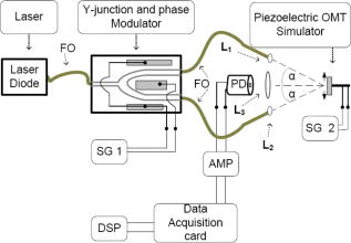

A linearly polarized adjustable power laser diode (FDL-638) is coupled by polarization maintaining an optical fiber to a combined Y-junction splitter and phase modulator (YJ-638), out of which extend two-phase maintaining optical fibers terminated with ferrule connector (FC) optical connectors.³⁰ The optical wavelength used is $λ = 638 nm$ . In order to collimate the spherical wave emerging from the FC connectors, visible to near-infrared FC focusing lenses (0.25 numerical aperture) were used in conjunction with thin, $6 - mm$ -diam lenses $(f = 72 mm)$ mounted in adjustable C-ring mount assemblies. Each beam is collimated and aligned, using lenses $L_{1}$ and $L_{2}$ , to interfere on a small area at angles of “ $α$ ” to the surface normal. For the results presented here, $α = 45 \deg$ .

The normally backscattered light intensity from the interference surface point can be collected by imaging lens $L_{3}$ , however an imaging lens was at first not used as it would have introduced an aperture which would increase the speckle size.³¹ In this paper, we therefore at first, while testing the device, did not include the imaging lens $L_{3}$ . Later, however, imaging lenses were introduced when using lower illuminating intensities.

Optoelectrical conversion of the time-varying speckle signal was performed using a low-capacitance Melles Griot photodiode (13dsi001 area $0.31 {mm}^{2}$ ). Amplification of the signal was performed using a low-noise Burr Brown operational amplifier (OPA637) in transimpedance gain configuration with a $20 M Ω$ resistor. To avoid electrical pickup, the casings of the photodiode, as well as the operational amplifier, were caged in a grounded metal case.

3.3.

Digital System Design

A $16 - bit$ National Instruments NI-USB 6221 analog to digital (ADC) converter was used to sample the time-varying optical signal at a sampling rate of $100 kHz$ . To ensure adequate sampling, $2 ω_{c} + ω_{\max} < 50 kHz$ , where $ω_{\max}$ is the highest frequency component of the motion, i.e., $\sim 200 Hz$ . Postprocessing of the data was performed with code written using The Mathworks, Inc., MatLab (vers.7)³² environment, employing the tools included in the basic software version. The sampling rate was chosen to be high enough to carry out signal processing operations digitally with sufficient bandwidth.

A variation of the method employed in previous papers^{10, 33, 34} to unwrap the phase signal was used to process the results presented in this paper. Integer multiples of $π$ are added or subtracted to the phase-wrapped signal $φ (t)$ depending on both the change of signs of successive quadrature sine $s_{s} (t)$ and cosine terms $s_{c} (t)$ . Discontinuities are obtained where the cosine term $s_{c} (t)$ is zero, i.e., goes from positive to negative or vice versa. The unwrapped phase signal is obtained when the values of discontinuities ( $- 1$ , 0, or 1) are convolved with $π$ values. The wrapped signal is then added to the result to yield the continuous phase signal. Scaling is preformed to convert the phase signal into a displacement signal using Eq. 12.

Our method of phase unwrapping for retrieving the true phase $ϕ_{d} (t)$ is as follows: First we determine the instances of zero values as described above. We then compare points at which zero crossing occurs with the sign of the wrapped signal’s slope. The multiple number of $π$ values is accumulated in a feedback loop leading to integer multiples of $π$ added or subtracted to the wrapped phase signal $ϕ_{w} (t)$ to determine the continuous phase signal, $ϕ_{d} (t)$ . Scaling, using Eq. 12, yields the displacement signal $d (t)$ .

4. System Performance and Evaluation

In this section we describe the experiments we carried out to calibrate the speckle interferometer, ensuring it can measure motions equivalent to those observed for OMT.

4.1.

Determining the Safe Region of Operation

The total optical power from each arm extending from the combined Y-junction and phase modulator was measured using a Newport 840-C optical power meter (serial no. 2269). By fitting the resultant light power versus current curve (see Fig. 3 ), we found the laser diode electro-optical transfer characteristic can be satisfactorily described, after reaching the threshold, using a third-order polynomial of the form

Eq. 17

P (i_{d}) = 4221.1 - 194.59 i_{d} + 2.7844 i_{d}^{2} - 0.0117 i_{d}^{3},

where

i_{d}

is the input current (mA), and

P (i_{d})

is the optical output power

(μ W)

.

Fig. 3

Experimental data for the $P (i_{d}$ ) curve with the a superimposed third-order polynomial (dotted) fitting the curve, and showing the required output power levels for MPE duration limits with 50.68 and 0% safety factors.

The SNR in the system has a bearing on the overall sensitivity of the system. The minimum resolvable displacements is dependant on the SNR, as shown which is itself dependant on both system parameters and also on the optical power of the speckle signal, which in turn is proportional to the laser output power. Using calculations of the MPE limit,²³ it is possible to identify a safe operational region where the safety guidelines are met and adequate SNR exists so as to allow reliable measurement of OMT vibrations.

When using the device in a clinical setting, each optical beam will have to be aligned so that they interfere on the sclera of the patient before measurement of the OMT can take place. Allowing (i) $270 s$ for alignment and (ii) $30 s$ to record OMT movement, the calculated MPE using Eq. 16 for both stages is presented in Table 1 . A second value for the MPE is also presented in Table 1 assuming operational safety factors of 50.68 and 17.56% of the MPE limit for the measurement and recording stages, respectively.

Table 1

Calculated MPE [Eq. 16] and proposed MPE with operational safety factor.

Experimental stage	MPE	MPE(With safety factor)
Measurement, $(t = 30 s)$	295.96 $μ W$	$150 μ W$ (50.68% of $295.96 μ W$ )
Alignment, $(t = 270 s)$	170.87 $μ W$	$30 μ W$ (17.56% of $170.87 μ W$ )

As stated, we assume that $\sim 100$ speckles are observed across our photodiode area. This implies that the maximum speckle diameter should be less than $60 μ m$ . Capturing the backscattered speckle field from out-test surface (see below) with a CCD camera (Fujifilm Finepix f460 with a Fujinon zoom lens, $f = 5.8 - 17.4 mm$ ) and a lens setup to magnify the field ( $f = 60 mm$ , lens diam $25 mm$ , magnification $M = 2$ ), we measured the speckle diameter to be between 51.3 and $56.8 μ m$ .

Figure 4a shows the SNR in decibels as a function of the laser power calculated using Eq. 13a assuming a 10% transmission factor, $T = 0.1$ , of the optics, and a 45% optical efficiency, $η = 0.45$ , for the photodiode. Three curves are presented using Danliker and Willemin’s assumptions^{25, 27} for heterodyne speckle interferometry and calculated assuming speckle diameters of 3.5, 35, and $350 μ m$ . Then, two special cases, when eye safety standards are met for safety factors of 50.68% (for $150 μ W$ illumination) and 0% (for $298 μ W$ illumination) are also shown for the case when the speckle diameter is $55 μ m$ . From the graph it can be seen that the 50.68% safety factor is met when the speckle signal has a value of $97.6 dB$ for the speckle diameter $55 μ m$ , as measured in our system. Figure 4b shows the corresponding logarithmic ${(d_{0})}_{\min}$ values predicted using Eq. 13b. As can be seen for the safe experimental laser power and speckle size, $10 \log_{10} [{(d_{0})}_{\min}] \approx - 116$ , corresponding to ${(d_{0})}_{\min} \approx 2.5 pm$ .

Fig. 4

(a) Theoretical (dashed) SNR calculations, using Eq. 13a, 13b logarithmic theoretical (dashed) minimum resolvable amplitude, using Eq. 13b, for speckle diameters of 3.5, 35, and $350 μ m$ and our measured speckle diameter of $55 μ m$ . The location of the MPE with operational safety factors (see Table 1) are included in both figures.

4.2.

Digital Simulation and Experimental Verification

The algorithm to process the speckle signal and perform phase unwrapping was implemented using Matlab, and in order to validate our software the demodulation process was numerically tested.

To examine the method, two simulated quadrature-shifted signals, a sine and a cosine version of the displacement signal of amplitude $2 μ m$ (pk-pk) and a frequency of $80 Hz$ , were generated assuming a wavelength of $638 nm$ and a standard sampling frequency of $100 kHz$ . The resulting arctangent of these two signals is a phase-wrapped version of the displacement signal. By applying the unwrapping technique as described above, the requisite number of integer values of $π$ required to unwrap the discontinuous signal is found. The result is the sinusoidal $80 Hz$ signal of amplitude $2 μ m$ (pk-pk).

In order to test the robustness of our software, additive white Gaussian noise was introduced, using the Matlab function AWGN, to the in-quadrature components before applying the arctangent function to the ratio of the sine and cosine terms. When the variance of the noise signal added to the quadrature signals was greater than 0.004, the onset of discontinuous unwrapping was observed to occur. In this case the technique applied a false phase increment or decrement to the wrapped signal.

The method was then applied to experimental data, the sampled output signal from the photodiode and amplifier, when a sinusoidal voltage was applied to a piezoelectric bimorph element (see below) to produce a $90 \pm 2 Hz$ sinusoidal signal of amplitude $1000 nm$ (pk-pk). The phase-wrapped phase signal from the arctangent of the ratio of the two quadrature signals is shown in Fig. 5a . The required phase additions are shown in Fig. 5b, and the resulting sinusoidal displacement is presented in Fig. 5c.

Fig. 5

(a) Phase-wrapped signal, Eq. 11, (b)required integer number of $π$ required to yield a continuous unwrapped signal, and (c) the resulting unwrapped phase signal $ϕ_{d} (t)$ .

Using this method, we have successfully demonstrated that our method can unwrap a discontinuous wrapped phase signal from two noisy quadrature signals. The resulting displacement signal, using Eq. 12, is found to have displacement amplitude of $977.06 nm$ (pk-pk). This is 2.3% below the expected amplitude of $1000 nm$ (pk-pk). The peak in the spectrum of the displacement signal occurs at $89.4 Hz$ , which is close to the $90 Hz$ driving frequency value.

4.3.

Calibrating the OMT Bimorph Simulators

Initially we tested our speckle system using lengths of Sensortech, Ltd., SM10-2501-00 piezoelectric bimorphs to simulate the microvibrations. The experimental setup is the same as that described in Sec. 3; however, we omitted the imaging lens, $L_{3}$ . As illustrated in Fig. 6a, simulator I consists of three bimorph elements of $25 - mm$ length and $1 - mm$ width, each with a rated sensitivity of $0.4 μ m ∕ V$ , extending from a rigid base. These are fixed normally to a curved rectangular piece of white, rough plastic of length $1 cm$ and width $0.5 cm$ . Attached to the side of this plastic is a small triangular prism. Applying a sinusoidal voltage to the outer bimorph elements causes a sinusoidal displacement. However, the central element, which is typically used to convert the displacement caused by the peripheral elements into a monitoring feedback electrical signal, acts to dampen the response of the outer elements. The weight of the rough plastic surface also reduces the rated sensitivity. In order to calibrate the actual response of the loaded system we used a Michelson interferometer, with the simulator prism positioned at one end of the interferometer arm, the damped response of simulator I was measured as $171.1 nm ∕ V$ .

Fig. 6

(a) Simulator I: sensitivity $171.1 nm ∕ V$ applied. (b) Simulator II: sensitivity $400 nm ∕ V$ .

Figure 7 shows two measured sinusoidal displacements at $110 \pm 1 Hz$ . The upper waveform has an amplitude of $2.7 μ m$ (pk-pk) and was driven using an applied voltage of $16.1 V$ (pk-pk). The lower waveform has an amplitude of $1.35 μ m$ (pk-pk) and was driven with an applied voltage of $7.9 V$ (pk-pk). These correspond to a measured response for the piezoelectric vibration simulator of $167.7 nm ∕ V$ for the upper and $170.6 nm ∕ V$ for the lower waveform. This in turn corresponds to errors of 0.5 and 0.25% in the measured response using the Michelson interferometer, which gives a measured response of $171.1 nm ∕ V$ .

Fig. 7

Measured displacement from the vibration simulator showing amplitudes and frequencies of (a) $2.7 μ m$ (pk-pk) and $109.1 Hz$ , and (b) $0.135 μ m$ (pk-pk) and $109.8 Hz$ .

Figure 8 gives the spectra of both of the signals shown in Fig. 7. The total number of samples used, $N$ , the sampled time interval SI, and the constant sampling rate $f_{s}$ , are given in the figure captions. Both have peak frequency components below $110 Hz$ , at 109.1 and $109.8 Hz$ . However, the spectral power of the peak component in Fig. 8b is less than that in Fig. 8a. This is as expected, as the amplitudes of both sinusoidal waveforms differ.

Fig. 8

Spectrum from $20 to 150 Hz$ of the waveforms in Fig. 7; peak frequency components occur at $110 Hz$ in both. (a) The spectrum of the waveform in Fig. 7a, with $N = 10^{6}$ samples, $S I = 10 s$ , $f s = 100 kHz$ , while (b) is the spectrum of the waveform in Fig. 7b, with 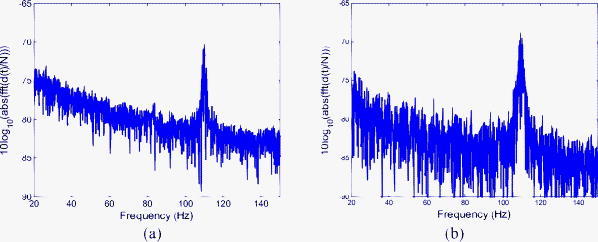$N = 1.1 \times 10^{6}$ , $S I = 11 s$ , $f s = 100 kHz$ .

The response of the vibration simulator was tested, using our speckle interferometer, by performing repeated measurements with the simulator vibrating at the following frequencies: 10, 30, 50, 70, 90, 110, 130, and $150 Hz$ . Throughout the experiments, the frequency reading had an error of $\pm 2 Hz$ . The piezoelectric elements were driven by pk-pk voltage amplitudes of $4.04 \pm 0.46 V$ , $7.8 \pm 0.118 V$ , $12.16 \pm 0.194 V$ , $16.15 \pm 0.8 V$ , and $20.98 \pm 0.04 V$ . The corresponding results estimated from the processed data are displayed in Table 2 . Note that the results presented do not cover the required OMT signal frequency or amplitude ranges.

Table 2

Simulator I. The measured displacement amplitude at increasing driving voltage and varying frequencies.

Drivingvoltage(V)	Expecteddisplacementamplitude(nm)	Frequency (Hz)
Drivingvoltage(V)	Expecteddisplacementamplitude(nm)	10 ±3	30 ±3	50 ±3	70 ±3	90 ±3	110 ±3	130 ±3	150 ±3
$20.98 \pm$ 0.04	3588	3168	3118	3190	3036	3302	3164	—	—
$16.15 \pm$ 0.8	2762	2444	2436	2426	2306	2458.2	2525	2588	—
$12.16 \pm$ 0.194	2080	1862.5	1906	1689.4	1901.4	1948.6	1948.2	2036	2000
$7.8 \pm$ 0.118	1334.4	1233.2	1240	1252.6	1267.2	1266.9	1298	1299	1352
$4.04 \pm$ 0.46	691.2	590	550	693.6	687.4	667	702.4	687.8	695

In calibrating simulator I using the Michelson interferometer, it was found that the central feedback probe reduced the simulator responsivity from the rated $400 nm ∕ V$ down to $171 nm ∕ V$ applied. In addition to this, simulator I was prone to breakdown, making reproducible measurement of displacements for the driving amplitudes and frequencies shown in Table 2 difficult. In order to more realistically simulate the full range of OMT-like movement in the human eye, we repeated the above experiments with a second simulator, simulator II, shown in Fig. 6b. Because it had been previously verified that the speckle interferometry system measurements agreed with those made using the Michelson bulk interferometer for simulator I, we immediately applied it to measure the response of simulator II over the complete range of amplitudes and frequencies associated with OMT. A single, undamped length of Sensortech, Ltd., piezoelectric bimorph material (SM10-2505-00), with a rated sensitivity of $400 nm per volt$ applied, was employed. A small sample of rounded white plastic was attached to the end to mimic the sclera. Under ideal conditions, applying a sinusoidal voltage of amplitude $5 V$ should result in a sinusoidal displacement of amplitude $2000 nm$ . To calibrate our device we tested it by applying sinusoidal signals with different amplitudes and frequencies to simulator II.

During the experiments describe above, we applied a driving current of $85 mA$ to the laser diode, which corresponds to a measured optical power of $598.5 μ W$ . This is above the safe limit of operation for use on a human eye. This high power level was employed in order to ensure a sufficiently high SNR to allow an unambiguous verification of the ability of the system to measure OMT-like motion. Table 3 shows the expected displacements and the experimentally resolved values of the amplitude for a range of frequencies. We note that measurements for the smallest signal, $50 nm$ (pk-pk), at the three lowest frequencies were not reproducible; however, measurements at $54 nm$ (pk-pk) were possible.

From Table 3 we can see our system is capable of measuring microvibrations over a wide range of amplitudes, from $100 to 2500 nm$ (pk-pk), and we have reproducibly measured microvibrations with amplitudes as low as $54 nm$ at $10 Hz$ . Using a similar optical technique²³ to measure OMT, the pk-pk amplitude of the OMT was measured to be centered at $728 nm$ , over a range from $598 to 903 nm$ . A number of investigations have indicated that peak OMT frequency for clinically normal patients occurs in the range of $88 \pm 7 Hz$ .^{1, 4, 35} Patients experiencing coma exhibit lower peak OMT frequency, between 40 and $60 Hz$ .¹⁵ The dashed region appearing in the center of the table of measured results, i.e., Table 3, includes both frequency and amplitude regions. Thus, we have demonstrated that a broad spectrum of frequencies, beyond those frequencies and amplitudes required to measure OMT, can be measured using our system.

4.4.

Test Using OMT Simulator II with a Wet Surface

The optically rough surface on the simulator was wet using a commonly available eye drop solution (brolene propamidine) to simulate water (tears) on the surface of the eye. In this way, the effects, if any, of tears on the recording of OMT signals using this optical system was examined.

Introducing the eye drop solution had no apparent effect on the measured result using the system. It remained possible to resolve a $684.48 nm$ (pk-pk) amplitude signal at $88.9 Hz$ signal using simulator II [see Figs. 9a and 9b ]. From the amplitude of the driving signal and the responsivity of the piezoelectric simulator, we expect a displacement of $698.1 nm$ ; thus, our measured result disagrees by only 1.9%.

Fig. 9

(a) Measured $684.48 nm$ (pk-pk) amplitude signal from a wet surface, and (b) signal spectrum showing peak at $88.9 Hz$ . $N = 1.1 \times 10^{6}$ samples, $S I = 11 s$ , $f s = 100 kHz$ .

Real tears are dynamic in the sense that the volume and density are likely to vary between patients. This simple experiment was carried out by wetting the rough surface to mimic the effects of teardrops. However, based on these results for static droplets, it appears that wetting is not likely to cause any significant operational issues in measuring OMT using this optical system.

4.5.

System Test Safe Light Levels

As stated earlier, the measurements presented so far result from illuminating the rough surface with $598.5 μ W$ of laser radiation. It is intended to illuminate the sclera of the eye. However, following the predictions of Eq. 16, accidental exposure of the retina can last less than $2 s$ at this intensity level before permanent damage occurs. In order to demonstrate that our device can operate at “eye safe” exposure levels and still measure OMT like microvibrations, we reduced the driving current in the laser so that it emits only $180 μ W$ of light. This is equivalent to a safety factor of 60.82% of the MPE, assuming a $30 s$ exposure in the recording stage (see Table 1). However, reducing the optical power also has the effect of reducing the SNR of the optical signal. As a consequence of this change, it was observed experimentally that the required interference fringes could no longer be successfully resolved.

To overcome this difficulty we first implemented two different unit magnification single-lens imaging systems using two different imaging lenses, $L_{3}$ ( $f = 10 mm$ , lens $diam = 7.5 mm$ , and $f = 20 mm$ , lens $diam = 15 mm$ ). As shown in Fig. 1 these were inserted appropriately between the rough surface and the photodiode. Attempts to measure microvibrations produced by simulator II were made but proved unsuccessful, as it remained impossible to resolve the interference fringes. Finally, an imaging lens $L_{3}$ ( $f = 35 mm$ , lens $diam = 25 mm$ ) was used to produce a system of magnification of $M = 2$ , and the interference fringes were resolved. Figure 10a shows the resulting measured noisy $647 nm$ (pk-pk) microvibration signal. The measured amplitude is 5.98% below the expected pk-pk amplitude of $688.89 nm$ . Figure 10b is the corresponding spectrum which contains a peak at $88.1 Hz$ .

Fig. 10

(a) Measured $647 nm$ (pk-pk) signal at measured using $180 μ W$ of illuminating light, and (b) signal spectrum showing peak at $88.1 Hz$ . $N = 10^{6}$ samples, $S I = 10 s$ , $f s = 100 kHz$ .

To perform an in vivo measurement using this lower power level one might proceed in a constrained manner, as follows: Suppose it is found necessary to use an exposure of $180 μ W$ for $30 s$ in order to record sufficient signal in order to accurately estimate OMT movements, then the device can be aligned for up to $270 s$ prior to measurement using a $30 - μ W$ signal with a safety factor of 17.56% of the MPE. In this case the eye is exposed to a total time-averaged intensity of $45 μ W$ . The requirement for eye safety is met as it is below the MPE for an exposure of $300 s$ at $166.4 μ W$ . Thus, this device is capable of measuring OMT-like movements using illumination intensities over exposure times which adhere to the safety requirements for accidental exposure of the retina.

4.6.

Estimation of System SNR

Operating our device, without any signal applied to simulator II and with all the background light sources turned off, we processed the recorded data to estimate the background noise of the system. The rough surface was illuminated with $598.5 μ W$ of laser radiation. At this power we found the best fit equation describing the noise from the resulting output of our system is

Eq. 18

N (f) = 214.5 - 270.64 {(2 π f)}^{0.0152} .

Figure 11 shows the resulting measured noise spectrum and the superimposed equation [Eq. 18], describing the background noise. The measured noise has contributions from the optics, thermal, flicker, and optoelectronic detector shot noise, as well as noise introduced by erroneous phase additions during phase unwrapping.

Fig. 11

Showing the background noise spectrum over the spectral region of interest. $N = 4 \times 10^{6}$ samples, $S I = 40 s$ , $f s = 100 kHz$ .

Table 3

Simulator II. Measured displacement amplitude at increasing driving voltage and varying frequencies.

Drivingvoltage(V)	Expecteddisplacementamplitude(nm)	Frequency (Hz)
Drivingvoltage(V)	Expecteddisplacementamplitude(nm)	10 ±2	30 ±2	50 ±2	70 ±2	90 ±2	110 ±2	130 ±2	150 ±2	170 ±2
6.24	2500	2464	2480	2280	2366	2452	2555	2780	2400	2502
5	2000	1976	1851	1830	1922	1994	2010	2260	2110	2180
3.74	1500	1380	1440	1320	1440	1450	1733	1920	1370	1534
2.5	1000	920	925	928	911	1034	1063	1143	1020	1185
1.24	500	583	491	471	497	449	492	599	483	310
0.74	300	322	301	299	247	304	349	315	320	334
0.50	200	211	216	200	2155	221	196	200	201	217
0.24	100	84	94	79.5	140	90	110	92	136	115
0.12	50	—	—	—	63	54	56	63	58	70

In Sec. 4.1 the optical SNR for a speckle system was given in Fig. 4a, calculated using Eq. 13a, while the corresponding minimum detectable displacement was presented in Fig. 4b using Eq. 13b. Having measured the speckle size in our system to be between 51.3 and $56.8 μ m$ , we assume a typical speckle diameter of $55 μ m$ . Assuming illumination of a rough surface with $598.5 μ W$ , Figs. 4a and 4b indicate an SNR of $+ 98 dB$ and a corresponding $10 \log_{10} [{(d_{0})}_{\min}] \approx - 118$ corresponding to ${(d_{0})}_{\min} \approx 1.6 pm$ . If only this type of noise were present we should be able to measure a signal of this size. However, in the experimental results presented in this paper we have succeeded in measuring only microvibrations with amplitudes down to $\sim 54 μ m$ (pk-pk). Clearly other, more dominant sources of noise exist in our system. While we might expect to significantly improve the system performance through the use of appropriate signal processing tools, it is unlikely that a noise floor corresponding to ${(d_{0})}_{\min} \approx 1.6 pm$ can in practice be achieved.

Let us analyze one of the typical results presented above. Figure 9b shows a measured spectrum using simulator II with $598.5 μ W$ , which includes a $684.48 nm$ (pk-pk) $88.9 Hz$ microvibrations signal. The measured rough surface is a wet surface and measurements took place under low-ambient-light conditions. From the figure the peak appearing as the input microvibration frequency has a value of about $- 72$ . From the same spectrum, we estimate that in the worst case the corresponding background noise floor value is about $- 82$ , which agrees well with the corresponding estimate using Eq. 18. The difference of $\sim 10$ between the noise floor and the peak at $88.9 Hz$ clearly corresponds to the effect of the OMT-like signal. Therefore, in this case the $SNR = 10$ , i.e., the ratio of the signal displacement to the random noise floor displacement at this frequency is 10. Because our input signal has a pk-pk amplitude of $684.48 nm$ , it appears that our noise floor in this case corresponds to $\sim 68 nm$ .

What other types of noise may be present in the system? One type of opto-electronic noise commonly encountered in low-frequency measurements is flicker noise, sometimes referred to as pink noise or $1 ∕ f$ noise. In this case, as implied, the spectral power density of the noise varies in inverse proportion to the frequency. As we are dealing with relatively low-frequency components, in the context of the electronic circuits used, we expect a contribution to the noise spectrum of this generic form. Other types of noise sources present may include ambient lighting and/or erroneous phase additions during unwrapping. We note that the experimental data which forms the basis of our estimation for the background noise in Eq. 18 was obtained under dark room conditions.

5. Discussion and Conclusions

We began this paper by reviewing the significance of the smallest and highest frequency of the three fixational eye movements, ocular microtremor, OMT. A noncontact measurement device for measuring eye movements, without the need to anaesthetize or make contact with the patient’s eyes, is shown to be useful. In a clinical setting, it could be used to diagnose several conditions, but prior to that, such a tool could help produce a better understanding of the link between several serious medical conditions and OMT. A noncontact system is desirable to allow greater convenience and patient acceptability in the clinical environment. It is also accurate to state that for vision scientists, a practical and viable method of measuring OMT noninvasively would be welcome.

In this paper we have described the design and development of a compact and portable fiber-based interferometer to measure OMT. The physical size of the system has been greatly reduced, compared to that of a bulk optical system, using optical components coupled together using optical fibers. This has resulted in a compact and easily portable system. We have tested this device, measuring in-plane motion of a rough surface using piezoelectric bimorph elements to provide calibrated test vibrations. The measurement of microvibrations over a range of amplitudes and frequencies, larger than those required to measure OMT, i.e., from $100 to 2500 nm$ (pk-pk), and over $10 to 170 Hz$ , has been demonstrated. In addition to this, it has been shown that the system can perform measurements while operating at safe illumination intensities for which accidental exposure of the retina will not causing permanent damage. A simple experiment was performed, the rough surface being wet to mimic the effects of static teardrops, and no operational problems using the optical method were observed. Therefore, a portable device capable of measuring OMT noninvasively and safely was implemented and tested.

In the course of this project we considered the effects of the speckle diameter and illuminating intensity on the SNR of the system. The background noise in the system was examined for practical cases. For the results presented in this paper, little or no digital signal processing, i.e., filtering, was carried out on the captured data. Addressing this issue alone should significantly improve the quality of the results, and thus SNR obtainable using this system.

For this device to be realized as a clinical tool for in vivo use by clinicians, several practical issues must be addressed. Local ethics board approval will be required before any in vivo test may be carried out. To measure the OMT using the system described here, it will be necessary to either isolate or measure simultaneously any head movement relative to the eye.

Future work will involve extending and modifying the above system to enable binocular OMT measurement and/or simultaneous vertical and horizontal displacement measurement. Isolating the recorded OMT signal from other signals, such as residual head movement, environmental vibrations, and cardiac pulse, could be accomplished by using a second device to accurately measure large-scale head movements at a stationary fixed reference point (e.g., bridge of the nose). This could be combined with an electrocardiogram (ECG) to filter out unwanted pulse signals. This could increase the number of possible applications of this method as a clinical diagnostic tool.

Acknowledgments

We acknowledge the support of Enterprise Ireland and Science Foundation Ireland through the Research Innovation, Proof of Concept Funds, and the Basic Research and the Research Frontiers Programs. We also thank the Irish Research Council for Science, Engineering and Technology. In addition, we recognize the support and contribution of Mercer’s Institute for Research on Ageing (MIRA) and the Medical Physics and Bioengineering Department at St. James’s Hospital to this project.

References

1.

D. Coakley, Minute Eye Movement and Brainstem Function, CRC Press, Boca Raton (1983). Google Scholar

2.

F. H. Adler and R. Fliegelman, “The Influence of fixation on visual acuity,” Am. J. Optom. Arch. Am. Acad. Optom., 12 475 –483 (1934). 0002-9408 Google Scholar

3.

M. P. Lord and W. D. Wright, “Eye movements during monocular fixation,” Nature (London), 162 25 –26 (1948). 0028-0836 Google Scholar

4.

N. F. Sheahan, D. Coakley, F. Hegarty, C. Bolger, and J. F. Malone, “Ocular microtremor measurement system: Design and performance,” Med. Biol. Eng. Comput., 4 205 –212 (1993). 0140-0118 Google Scholar

5.

F. Ratliff and L. A. Riggs, “Involuntary motions of the eye during fixation,” J. Exp. Psychol., 40 687 –701 (1950). 0022-1015 Google Scholar

6.

R. W. Ditchburn and B. L. Ginsborg, “Involuntary eye movements during fixation,” J. Physiol. (London), 119 1 –17 (1953). 0022-3751 Google Scholar

7.

G. C. Higgins and K. F. Stultz, “Frequency and amplitude of ocular tremor,” J. Opt. Soc. Am., 43 1136 –1140 (1953). 0030-3941 Google Scholar

8.

C. Bolger, N. Sheahan, D. Coakley, and J. Malone, “High Frequency eye tremor: reliability of measurement,” Clin. Phys. Physiol. Meas., 13 151 –159 (1992). 0143-0815 Google Scholar

9.

A. Spauschus, J. Marsden, D. M. Halliday, J. R. Rosenberg, and P. Brown, “The origin of ocular microtremor in man,” Exp. Brain Res., 126 556 –562 (1999). 0014-4819 Google Scholar

10.

G. Boyle, D. Coakley, and J. F. Malone, “Interferometry for ocular microtremor measurement,” Appl. Opt., 40 167 –175 (2001). https://doi.org/10.1364/AO.40.000167 0003-6935 Google Scholar

11.

G. W. Hebbard and E. Marg, “Physiological nystagmus in the cat,” J. Opt. Soc. Am., 50 151 –155 (1960). 0030-3941 Google Scholar

12.

A. R. Shankovich and J. G. Thomas, “Ocular microtremor: An index of motor unit activity and of the functional state of the brain stem,” J. Physiol. (London), 238 36P (1974). 0022-3751 Google Scholar

13.

V. Golda, P. Petr, F. Cerak, V. Rozsival, and J. Sverak, “Oculomicrotremor and the level of vigilance,” Sb. Ved. Pr. Lek. Fak. Karlovy University Hradci Kralone, 24 77 –83 (1981) Google Scholar

14.

D. Coakley and J. G. Thomas, “The ocular microtremor record as a potential procedure for establishing brain death,” J. Neurol. Sci., 31 199 –205 (1977). 0022-510X Google Scholar

15.

D. Coakley and J. G. Thomas, “The ocular microtremor as a prognosis of the unconcious patient,” Lancet, 5 512 –522 (1977). 0140-6736 Google Scholar

16.

S. Bojanic, T. Simpson, and C. Bolger, “Ocular microtremor: a tool for measuring depth of anaesthesia?,” Br. J. Anaesth., 86 519 –522 (2001). 0007-0912 Google Scholar

17.

L. G. Kevin, A. J. Cunningham, and C. Bolger, “Comparison of ocular microtremor and bispectral index during sevoflurane anaesthesia,” Br. J. Anaesth., 89 551 –555 (2002). 0007-0912 Google Scholar

18.

M. Heaney, L. G. Kevin, A. R. Manara, T. J. Clayton, S. D. Timmons, J. J. Angel, K. R. Smith, B. Ibata, C. Bolger, and A. J. Cunningham, “Ocular microtremor during general anesthesia: results of a multicenter trial using automated signal analysis,” Anesth. Analg. (Baltimore), 99 775 –780 (2004). 0003-2999 Google Scholar

19.

C. Bolger, S. Bojanic, N. F. Sheahan, D. Coakley, and J. F. Malone, “Ocular microtremor in patients with idiopathic Parkinson’s disease,” J. Neurol., Neurosurg. Psychiatry, 66 528 –531 (1999). 0022-3050 Google Scholar

20.

C. Bolger, S. Bojanic, N. F. Sheahan, J. F. Malone, M. Hutchinson, and D. Coakley, “Ocular microtremor (OMT): a new neurophysiological approach to multiple sclerosis,” J. Neurol., Neurosurg. Psychiatry, 68 639 –642 (2000). 0022-3050 Google Scholar

21.

C. Bolger, S. Bojanic, N. F. Sheahan, D. Coakley, and J. F. Malone, “Effects of age on ocular microtremor activity,” J. Gerontol., Ser. A, 56A M386 –M390 (2001). 1079-5006 Google Scholar

22.

S. Martinez-Conde, S. L. Macknik, and D. H. Hubel, “The role of fixational eye movements in visual perception,” Nat. Rev. Neurosci., 5 229 –240 (2004). https://doi.org/10.1038/nrn1348 1471-003X Google Scholar

23.

G. Boyle, “Ocular microtremor, non-contacting measurement and biophysical analysis,” Trinity College, (1998). Google Scholar

24.

J. A. Leendertz, “Interferemetric displacement measurements on scattering surfaces utilizing speckle effects,” J. Phys. E, 3 214 –218 (1970). https://doi.org/10.1088/0022-3735/3/3/312 0022-3735 Google Scholar

25.

R. Dandliker and J.-F. Willemin, “Measuring microvibrations by hetrodyne speckle interferometry,” Opt. Lett., 6 165 –167 (1981). 0146-9592 Google Scholar

26.

I. S. Gradshteyn and I. M. Ryzhik, Table of Integrals, Series, and Products, 4th ed.Academic Press, London (1980). Google Scholar

27.

J.-F. Willemin and R. Dandliker, “Measuring amplitude and phase of microvibrations by hetrodyne speckle interferometry,” Opt. Lett., 8 102 –104 (1983). 0146-9592 Google Scholar

28.

F. C. Delori, R. H. Webb, and D. H. Slineey, “Maximum permissible exposure for ocular safety (ANSI 2000), with emphasis on ophthalmic devices,” J. Opt. Soc. Am. A, 24 1250 –1265 (2007). https://doi.org/10.1364/JOSAA.24.001250 0740-3232 Google Scholar

29.

IEC International Standard 825–1, International Electrotechnical Commission, Geneva ( (1993) Google Scholar

30.

GmbH, G.C.T. (2005) http://www.guidedcolour.de/main.html Google Scholar

31.

D. P. Kelly, J. E. Ward, U. Gopinathan, and J. T. Sheridan, “Controlling speckle using lenses and free space,” Opt. Lett., 32 3394 –3396 (2007). https://doi.org/10.1364/OL.32.003394 0146-9592 Google Scholar

32.

, (2007) http://www.mathworks.com/products/matlab/ Google Scholar

33.

O. Sasaki and K. Takahashi, “Sinusoidal phase modulating inteferometer using optical fiber for displacement measurement,” Appl. Opt., 27 4139 –4142 (1988). 0003-6935 Google Scholar

34.

T. Suzuki, O. Sasaki, K. Higuchi, and T. Maruyama, “Real time displacement measurement in sinusoidal phase modulating interferometry,” Appl. Opt., 28 5270 –5274 (1989). 0003-6935 Google Scholar

35.

C. Bolger, S. Bojanic, N. F. Sheahan, D. Coakley, and J. F. Malone, “Dominant frequency content of ocular microtremor from normal subjects,” Vision Res., 39 1911 –1915 (1999). 0042-6989 Google Scholar

Citation Download Citation

James Patrick Ryle, Mohammed Ali Al-Kalbani, Niamh Collins, Unnikrishnan Gopinathan, Gerard Boyle, Davis Coakley, and John T. Sheridan "Compact portable ocular microtremor sensor: design, development and calibration," Journal of Biomedical Optics 14(1), 014021 (1 January 2009). https://doi.org/10.1117/1.3083435

Published: 1 January 2009

Access the abstract

JOURNAL ARTICLE
12 PAGES

DOWNLOAD PAPER SAVE TO MY LIBRARY

GET CITATION

CITATIONS

Cited by 12 scholarly publications.

Explore citations on Lens.org

RIGHTS & PERMISSIONS

Get copyright permission Get copyright permission on Copyright Marketplace

KEYWORDS

Eye

Speckle

Signal to noise ratio

Calibration

Safety

Sensors

Signal processing

1.

Introduction

2.

Principle of Operation

Fig. 1

Eq. 1

Eq. 2

Eq. 3

Eq. 4

Eq. 5

Eq. 6

Eq. 7

Eq. 8

Eq. 9

10.

Eq. 11

Eq. 12

Eq. 13a

Eq. 13b

3.

Design and Development of a Noncontact OMT Sensor

3.1.

Laser Safety Standards

Eq. 14

Eq. 15

Eq. 16

3.2.

Compact Optical System Design

Fig. 2

3.3.

Digital System Design

4.

System Performance and Evaluation

4.1.

Determining the Safe Region of Operation

Eq. 17

Fig. 3

Table 1

Fig. 4

4.2.

Digital Simulation and Experimental Verification

Fig. 5

4.3.

Calibrating the OMT Bimorph Simulators

Fig. 6

Fig. 7

Fig. 8

Table 2

4.4.

Test Using OMT Simulator II with a Wet Surface

Fig. 9

4.5.

System Test Safe Light Levels

Fig. 10

4.6.

Estimation of System SNR

Eq. 18

Fig. 11

Table 3

5.

Discussion and Conclusions

Acknowledgments

References

Show All Keywords

Keywords/Phrases

Search In:

Publication Years