2.1.

Microscopes

For epifluorescence measurements, we used either an AxioObserver.Z1 or an Axiovert 200M (both Zeiss, Jena, Germany) equipped with a $40\times ∕1.2\mathrm{W}$ C-Apochromat or a $63\times ∕1.4$ Oil Plan-Apochromat, and the Zeiss-filter sets 10, 49, 38 HE, 43, and 32. The AxioVision software (Zeiss, V. 4.6 or 4.4) was used to operate the microscope and readout of the charge-coupled device (CCD)-camera (AxioCam MRm, pixel size $6.45\mu \mathrm{m}\times 6.45\mu \mathrm{m}$ , $1388\times 1040\text{pixels}$ or AxioCam HR, $6.7\mu \mathrm{m}\times 6.7\mu \mathrm{m}$ , $1300\times 1030\text{pixels}$ ). The illumination source was either a $120\text{-}\mathrm{W}$ metal halide short-arc lamp (Exfo, Mississauga, Canada) or a xenon arc lamp (XBO 75).

For structured illumination measurements, the ApoTome-slider was introduced into the field-stop plane of one of the above microscopes. Thereby, one of two available rectangular-shaped gratings was inserted into the field-stop plane: either a grid with ${\nu }_{\mathrm{VH}}=17.5\text{lines}∕\mathrm{mm}$ or a grid with ${\nu }_{\mathrm{VL}}=35\text{lines}∕\mathrm{mm}$ . “VH” stands for the designated use with “high” magnification objectives, and “VL” stands for the designated use with “low” magnification objectives in an Axiovert microscope. If the $63\times ∕1.4$ Oil Plan-Apochromat objective and $\lambda =500\mathrm{nm}$ are used, the corresponding normalized grid frequencies are ${\widehat{\nu }}_{\mathrm{VH}}=0.15$ and ${\widehat{\nu }}_{\mathrm{VL}}=0.29$ . Grid phase and focus calibration were performed prior to each experiment. For a $z$ -stack, 60 sectioned images at $100\text{-}\mathrm{nm}$ distance were taken. The acquired image stacks were exported as $16\text{-}\text{bit}$ TIFF images.

For cLSM measurements, the laser scanning unit LSM 510 (Zeiss) was attached to an Axiovert 100M that was equipped with the same objectives as above. The $488\text{-}\mathrm{nm}$ laser line was used for excitation. Pinhole calibration was performed before every experiment. The pixel size was set to $71\mathrm{nm}\times 71\mathrm{nm}$ for the measurement of point-spread functions (PSFs), or to $285\mathrm{nm}\times 285\mathrm{nm}$ for measuring subresolution homogeneous fluorescent layers. Sixty images at $100\mathrm{nm}$ axial distance were taken. The cLSM setup was controlled by the LSM 510 software (V 3.2). Images were taken at $12\text{bit}$ and exported as $12\text{-}\text{bit}$ TIFF files.

2.2.

Test Objects: Fluorescent Beads, Layers, and Thin Dendrites

InSpeck Green microspheres $(175\pm 5\mathrm{nm})$ with a fluorescence coating ( ${\lambda }_{\mathrm{ex}}=505\mathrm{nm}$ , ${\lambda }_{\mathrm{em}}=515\mathrm{nm}$ , Invitrogen, Karlsruhe, Germany) were used to measure PSFs. The experimentally determined PSFs are the result of the convolution of the test object (bead) with the imaging system transfer function and thus always affected by the test object's dimension. While the PSFs’ axial extensions are nearly unaffected by this convolution, the lateral extensions are slightly higher than the actual microscope’s resolution in the given high NA regime. The beads used are hence a compromise with respect to the available signal. The beads were dissolved in 70% ethanol, pipetted onto a cover slip, and allowed to dry. Mounting medium ( $15\mu \mathrm{L}$ Component E, Invitrogen, Karlsruhe, Germany) was then added and gently sealed by covering it with an object slide.

In order to measure how a subresolution homogeneous fluorescent layer in the object plane is imaged, we used reference layers fabricated as $100\text{-}\mathrm{nm}$ thick fluoresceine/perylenediimid layers, which had a refractive index of $n_{\mathrm{D}}\approx 1.59$ .¹⁶

As test objects for anisotropic axial resolution, we prepared cell-cultures with small, straight-grown dendrites. The cell-culture preparation was done as described by Gennerich and Schild.¹⁷ Measurements were carried out within five to ten days after plating. Prior to the experiments, the cultures were loaded for $15\min$ with $100\mu \mathrm{M}$ calcein-acetoxymethyl ester (Invitrogen, ${\lambda }_{\mathrm{cm}}=514\mathrm{nm}$ at pH 7.8), which was dissolved in dimethylsulfoxide (DMSO) and Pluronic F-127 (Invitrogen). The final concentrations of DMSO and Pluronic F-127 did not exceed 0.5 and 0.1%, respectively.

2.3.

Tissue Preparation

Larvae of Xenopus laevis (stage 54 and older)¹⁸ were chilled in a mixture of ice and water and decapitated as approved by the Göttingen University Committee for Ethics in Animal Experimentation. A block of tissue containing the anterior two-thirds of the olfactory bulb was extirpated and glued onto the stage of a vibroslicer (VT 1000S; Leica, Bensheim, Germany). A tissue slice of $\approx 300\text{-}\mu \mathrm{m}$ thickness containing the glomerular layer was cut out and transferred to a patch clamp setup. The whole cell configuration was established, and the cell was loaded $\approx 1\min$ with Alexa Fluor 488 biocytin (Invitrogen). After another $20\min$ , the tissue block was turned upside down and imaged under the ApoTome and the cLSM by using an axial stepwidth of $1.5\mu \mathrm{m}$ (overview) or $0.45\mu \mathrm{m}$ (selected positions).

Multicolour tissue visualization was prepared in four subsequent steps. (i) For tracing olfactory nerve fibers, some crystals of Alexa Fluor 488 biocytin were placed into the cut olfactory nerve of chilled tadpoles and the lesion was closed with cyanoacrylic glue (Roti-Coll 1, Roth, Karlsruhe, Germany). The tadpole was decapitated $3\mathrm{h}$ later, as described above, and a block of tissue containing the olfactory nerves and the anterior two-thirds of the brain were cut out and kept in a bath solution. (ii) A solution containing Alexa Fluor 546 biocytin was injected into the olfactory tract, and the tissue was incubated for another $2\mathrm{h}$ . Then, the tissue block was fixed in 4% formaldehyde in $0.1\mathrm{M}$ phosphate buffered saline (PBS) for $\approx 2\mathrm{h}$ , washed in PBS $(3\times 10\min )$ , embedded in agarose, glued onto the stage of a vibroslicer (VT 1000S; Leica, Bensheim, Germany), and cut into slices of $70\text{-}\mu \mathrm{m}$ thickness. (iii) The slices were incubated in PBS containing 1% bovine serum albumin (BSA) for $30\min$ at room temperature. Then, they were incubated overnight in Alexa Fluor 647 Phalloidin (Invitrogen) ( $5\mu \mathrm{L}$ from methanol stock solution) in $200\mu \mathrm{L}$ of PBS with 1% BSA. (iv) For further staining with $4^{\prime }$ ,6-diamidino-2-phenylindole [(DAPI) Invitrogen], the slices were washed $3\times 10\min$ in PBS and incubated for $15\min$ in a mixture of $1\mathrm{mL}$ of PBS and $2\mu \mathrm{L}$ of DAPI stock solution. After washing in PBS $5\times 10\min$ , they were mounted on object slides with DAKO Cytomation (Hamburg, Germany) Fluorescence Mounting Medium S3023.

2.4.

Solutions

2.5.

Analysis

Data analysis was done by using programs written in Matlab. In order to determine the PSFs, single-bead images were cropped. The lateral resolution was obtained from a 2-D–Gaussian fit to the center-of-gravity (COG) plane. The axial resolution was obtained from a 1-D skewed Gaussian fit to the column containing the COG. ${\chi }_{\mathrm{R}}^2$ did not improve if the theoretically more precise descriptions for the axial and lateral PSF behavior are used.²⁰ The cropped PSFs were then aligned to the COG with subpixel precision and summed up.

Our Matlab Sectioned Image Property chart (SIPchart) analysis¹⁶ allowed freely selectable binning filters and free choice of a number of fit functions. Thus, ApoTome data were fitted by using a skewed Gaussian, where the $z$ coordinate was assumed to follow $z^{\prime }=z\exp (-sz)$ , with $s$ being the skew factor, and $I=I_0\exp (-z^{\prime 2}∕2{\sigma }^2)$ . cLSM data were fitted by using a skewed Lorentzian with $I=I_0[{\sigma }^2∕({\sigma }^2+4z^{\prime 2})]$ .

3.1.

Lateral Resolution

We measured the PSFs of fluorescent beads by using a $63\times ∕1.4$ Oil Plan-Apochromat objective (Zeiss) in order to compare the resolving power of the ApoTome with epifluorescence and confocal microscopes.²¹ The radial and the axial projections of the resulting PSFs are shown in Fig. 2 for epifluorecence [Fig. 2a], for the ApoTome with the VH grid or VL grid [Figs. 2b and 2c], and for the cLSM [Fig. 2d]. There is no significant difference between the ApoTome and the standard epifluorescence microscope with regard to lateral resolution, whereas the cLSM’s PSF was slightly broader. Two noncommercial implementations of structured illumination^{2, 22} are reported to have a lateral resolution higher than this. Note that SIM as realized in the ApoTome is not a linear-shift invariant system [cf. Eq. 2]. Thus, it is not possible to describe the process of obtaining an ApoTome image in terms of the PSF for the general case. To this end, a set of fluorescent test samples containing all spatial frequencies in a defined manner would be required. Karadaglic and Wilson¹³ showed that in the case of defocus the features around the frequency $\nu$ are enhanced. This effect appears in the interaction between the object’s zeroth spatial frequency and the frequencies close to $v$ . The PSF is still a useful measure of the resolution though less informative when imaging complex structures.

Fig. 2

(a–d) Lateral and axial PSFs obtained from $175\pm 5\mathrm{nm}$ green fluorescent beads embedded in component E. PSFs were produced by manually selecting $\gtrsim 100$ bead images for every imaging mode, aligning them with subpixel precision to their center of gravity, and calculating the mean. The axial resolutions in the cLSM determined with $d_{\mathrm{p}}=1\mathrm{A.U.}$ and in the ApoTome determined with the VL grid are similar. VH, ApoTome low sectioning $({\widehat{\nu }}_{\mathrm{VH}}=0.15)$ ; VL, ApoTome high sectioning $({\widehat{\nu }}_{\mathrm{VL}}=0.29)$ ; EF, conventional epifluorescence. See text for further explanation.

The resolution of the cLSM is determined by the size of the emission pinhole, and for maximally closed pinholes, theory predicts an improvement of $\sqrt{2}$ over epifluorescence,²³ where 95% of the in-focus light is rejected by the pinhole. A pinhole size of $d_{\mathrm{p}}=1$ Airy unit (A.U.) is often considered a good compromise between resolution and detected light intensity.²⁴ If, in this case, the backfocal plane (BFP) is illuminated homogeneously, then the lateral resolution of the cLSM should outperform epifluorescence by ${\lambda }_{\mathrm{cm}}∕{\lambda }_{\mathrm{ex}}$ . In our measurements, the cLSM’s lateral resolution fell behind that of epifluorescence or the ApoTome: $d_{l,\mathrm{EF}∕\mathrm{VH}∕\mathrm{VL}}\cdot 1.1=d_{l,\mathrm{cLSM}}$ . This may be explained, first, by the Gaussian intensity profile in the BFP, which reduced the effective NA.²⁵ A second explanation is that the axial resolution is distributed spatially inhomogeneous (see below).

3.2.

Axial Resolution

It is customary to determine a microscope’s axial resolution with fluorescent beads. Fluorescently labelled biological objects are however often rather densely, almost homogeneously stained, so that a fluorescent layer would seem a more adequate test object to determine axial resolution. Here we start by using beads as test objects, and will then use subresolution homogeneous fluorescent layers.

The axial resolution determined with beads differed markedly in the three microscopes analyzed. The full-width-at-half-maximum (FWHM) values of the axial Gaussian fits (Fig. 2, lower row) clearly show (i) that the ApoTome’s axial resolution is better than that of the epifluorescence microscope, (ii) that the ApoTome’s axial resolution depends on the grid used, and (iii) that the ApoTome’s axial resolution with the VL grid is about the same as that of the cLSM (at a pinhole diameter of $d_{\mathrm{p}}=1\mathrm{A.U.}$ ). In conventional epifluorescence, the bead images show the characteristic butterfly-shaped side lobes as predicted by electromagnetic wave theory.²⁰ These are clearly reduced in the ApoTome. If the finer grid (VL) is used, then the ApoTome yields a 33% advantage over conventional epifluorescence and matches the cLSM’s resolution.

Figure 3 shows the axial resolution (i) of the cLSM as a function of the pinhole diameter, (ii) of the ApoTome equipped with the VH grid $({\widehat{\nu }}_{\mathrm{VH}}=0.15)$ , (iii) of the ApoTome equipped with the VL grid $({\widehat{\nu }}_{\mathrm{VH}}=0.29)$ , and (iv) of epifluorescence illumination determined with beads [Fig. 3a] and layers [Fig. 3b]. If the axial resolution was determined with beads, then the use of the ApoTome’s VH grid corresponds to $d_{\mathrm{p}}\approx 1.5\mathrm{A.U.}$ in the cLSM, whereas the use of the VL grid corresponds to $d_{\mathrm{p}}\approx 1\mathrm{A.U.}$ Certainly, with increasingly smaller pinhole sizes, there is a marked increase in resolution (e.g., $0.43\pm 0.14\mu \mathrm{m}$ at $d_{\mathrm{p}}=0.4\mathrm{A.U.}$ ). This outperforms the ApoTome’s best bead resolution. It can also be seen from Fig. 3 a that for large pinhole sizes $(d_{\mathrm{p}}⩾2\mathrm{A.U.})$ , the cLSM shows worse axial resolution than the epifluorescence microscope due to the Gaussian illumination of the BFP in the cLSM [i.e., due to the effect that the effective NA in the cLSM is lower than the nominal one, which is indicated on the objective barrel (here, 1.4)].

Fig. 3

Axial resolution as a function of the pinhole diameter determined by the use of fluorescent beads (a), and subresolution homogeneous fluorescent layers (b). If the pinhole is opened, then the axial resolution increases in a subproportional way in the case of using fluorescent beads. It increases almost linearly if fluorescent layers are used. The diameter of the pinhole $d_{\mathrm{p}}$ is given in A.U. as it appears back projected in the focal region. For comparison, the ApoTome resolution values are given as indicated. VH, ApoTome low sectioning $({\widehat{\nu }}_{\mathrm{VH}}=0.15)$ ; VL, ApoTome high sectioning 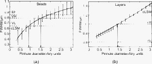$({\widehat{\nu }}_{\mathrm{VL}}=0.29)$ .

If the axial resolution is determined with subresolution homogeneous fluorescent layers, then the VL grid of the ApoTome will have about twice the resolution compared to the VH grid. This is expected from the twice-finer-grid structure and the corresponding cutoff frequency. Under these conditions, the ApoTome achieves a better resolution than the cLSM with a pinhole at minimum diameter [Fig. 3b]. For these comparisons, we took into account the bigger field of view of the cLSM by cropping a field of view corresponding to the size of the ApoTome’s field of view from the cLSM image. Because the axial resolution in the cLSM varied with the distance from the optical axis (see Section 3.3), the centerline of the crop stack was determined by the highest resolution.

3.3.

Spatial Inhomogeneity of Axial Resolution

To investigate the possibility that the axial resolution was spatially inhomogeneously distributed, one can either measure bead PSFs at multiple distances from the optical axis (which is rather impractical) or use SIPcharts.¹⁶ These are generated from image stacks of a subresolution homogeneous fluorescent layer.

The SIPchart intensity distribution clearly showed radial symmetry both for the cLSM [Fig. 4a ] and for the ApoTome [Fig. 4b]. Moreover, the axial resolution in the cLSM was highly correlated with the radial intensity distribution [Fig. 4c]. The symmetric shape can be ascribed to spherical and chromatic aberrations, while the off-axis resolution maximum can presumably be attributed to a slightly imperfect pinhole adjustment. Remarkably, there is a difference of $\approx 250\mathrm{nm}$ (22% or $\lambda ∕2$ ) between the best resolved regions at the intensity maximum and the worst resolved regions [see Fig. 4c]. Thus, the radial symmetry of and the change in axial resolution indicate that the specific position in the field of view in a cLSM image determines at which precision a subcellular structure can be resolved. Contrary to the cLSM, the ApoTome’s axial resolution appears to be quite homogeneous, the deviations being $⩽\lambda ∕10$ .

Fig. 4

(a–d) Extract of SIPcharts: a thin homogeneous fluorescent layer was recorded in a 3-D image stack, axial step size $100\mathrm{nm}$ , and subsequently processed to obtain SIPcharts, of which the extracts above directly compare illumination and resolution properties of the ApoTome (VH grid) and the cLSM system $(d_{\mathrm{p}}=1\mathrm{A.U.})$ . The maximum intensity $I_{\max }$ has a circular-symmetric shape in both imaging modes, which is ascribed to chromatic and spherical aberration. Without the application of a spatial filter, there remain stripe artifacts induced by improper phase shifts of the grid, intensity fluctuations, and stage movements during acquisition and bleaching. The blots in the ApoTome images stem from a residue on the grid, underlining the importance of keeping it perfectly clean. Values (insets) refer to binned data sets $\text{mean}\pm \mathrm{sd}$ over the whole field of view (ApoTome: $8\times 2$ binning mask to conserve the stripe pattern of the $1388\times 1040\text{pixels}$ image: one period of the grid pattern is sampled by $\approx 23\text{pixels}$ (VH grid) or $\approx 11.5\text{pixels}$ (VL grid), leading to an artifact stripe pattern of $3\times$ the grid pattern; cLSM: $6\times 6$ binning mask for a $512\times 512\text{pixels}$ image); objective: $63\times /1.4$ Oil Plan-Apochromat.

Interestingly, another feature of the ApoTome can be derived from the SIPcharts shown in Figs. 4b and 4d; both reveal an artifact stripe pattern, which may result from stage vibrations leading to nonstationary imaging of the grid into the sample, imprecise phase shifts of the grid, bleaching of the grid pattern into the sample, or intensity fluctuations of the illumination arc source. The AxioVision software includes a digital filter that removes certain spatial frequencies in the Fourier domain. We found that the so-called weak filter was the best to remove the stripe artifacts under most imaging conditions. But the SIPcharts produced with the “weak filter” setting led to a substantial loss in axial resolution, namely, $1.2\pm 0.03\mu \mathrm{m}$ versus $1.0\pm 0.02\mu \mathrm{m}$ (VH) and $0.69\pm 0.05\mu \mathrm{m}$ versus $0.61\pm 0.05\mu \mathrm{m}$ (VL). Certainly, it can be expected that spatial low-pass filtering reduces spatial resolution. Because the AxioVision filtering algorithms are not documented, the user applying a spatial filter to remove the stripe artifacts must find out, empirically, the impact of the filter used on axial resolution.

3.4.

Anisotropy of Resolution

The ApoTome’s grid-shaped illumination being 1-D modulated suggested that its axial resolution might by anisotropic. To test this, we measured the axial extensions of small and straight fluorescence-labeled neuronal dendrites in cell culture, taking the angle between dendrite and grid pattern as the parameter (Fig. 5 ). The lateral extensions of the dendrites were virtually independent of their orientation with respect to the grid [ $350\pm 5\mathrm{nm}$ (parallel) and $347\pm 5\mathrm{nm}$ (orthogonal), $\text{mean}\pm \mathrm{sd}$ ]. In contrast to that, the axial extension of dendrites oriented in a parallel way was significantly larger than that of dendrites oriented in an orthogonal way, with the angle dependency of the axial resolution being rather steep, assuming the value for orthogonal dendrites for less than $\alpha =3\mathrm{deg}$ (Fig. 5).

Fig. 5

Anisotropic resolution in the ApoTome. Straight-grown, smooth, fluorescence-labelled dendrites from cell cultures of olfactory bulb neurons of Xenopus laevis were recorded as image stacks at several angles to the grid pattern. In the example shown (a–d), the angle is $2.8\mathrm{deg}$ (a–c) raw images, right: illumination pattern giving the image to the left, and (d) processed images, right: color bar for (a–d). A 2-D Gaussian fit was applied to the corresponding image plane (either $xz$ or $yz$ plane) (e) An analysis of each dendrite reveals a rapidly increasing resolution with increasing angle to the grid. The lateral extension of the dendrites in the $xy$ plane does not depend on the angle between the dendrite and the grid. It was $0.350\pm 0.005\mu \mathrm{m}$ $(\text{mean}\pm \mathrm{sd})$ in case the dendrite was parallel (p) to the grid, and $0.347\pm 0.005\mu \mathrm{m}$ if it was orthogonal (o) to the grid (f) Normalized distribution of the axial extension of the dendrite tilted $1.8\mathrm{deg}$ obtained from $\gtrsim 300$ fits to the $xz$ plane. The Gaussian distribution of the observable resolution supports the hypothesis that the dendrites’ extensions are below the resolution limit.

3.5.

Deep-Tissue Imaging

Because it is of practical relevance how well an optical sectioning technique works within stained biological tissue, we stained mitral cells of the olfactory bulb with Alexa Fluor 488 biocytin through a patch pipette and imaged the same cells by using the cLSM 510 and the ApoTome (Fig. 6 ). Morphological details close to the surface of the tissue can be resolved equally well in the ApoTome and the cLSM (plane a of Fig. 6), but in greater depths (planes b and c of Fig. 6) the ApoTome images show increased blur and noise. In plane b, for instance, the image plane cutting a dendrite is well below the cell’s soma. The dendrite cut is clearly seen in both the ApoTome and the cLSM, but in addition, the ApoTome image shows a blurry spot, which is not seen in the cLSM image, reporting the noise originating from the soma above that plane; this is because the ApoTome, though taking into account out-of-focus light while calculating an optical section, does not remove the noise of out-of-focus light.²⁶ At imaging depths of several cell layers, the noise component becomes dominant in the ApoTome, preventing the acquisition of feature-rich images; at the same depth in the same preparation, the cLSM can still extract tiny structures (plane c of Fig. 6). This is of course due to out-of-focus photons being confocally suppressed in the cLSM. In the ApoTome in contrast, the grid pattern projected onto the focus plane is increasingly superimposed by scattered light at greater tissue depth. Moreover, its in-focus modulation is correspondingly attenuated with stronger staining; these effects are not taken into account by Eqs. 1, 2, 3.

Fig. 6

A mitral cell in the olfactory bulb loaded with Alexa Fluor 488 biocytin through a patch pipette. Maximum projections in (a) $xy$ , (b) $xz$ , and (c) $yz$ calculated from a stack of cLSM images. The color is used to code the $z$ coordinate (see color bar). In addition, images were taken from the same tissue volume with the ApoTome. (d) Comparison of ApoTome optical sections (left column) and cLSM sections (right column) taken at the planes a, b, and c as indicated in the maximum projections ( $\mathrm{a}=10\mu \mathrm{m}$ , $\mathrm{b}=27\mu \mathrm{m}$ , $\mathrm{c}=58\mu \mathrm{m}$ ). At $z=27\mu \mathrm{m}$ , the ApoTome image is markedly corrupted from noise caused by the brightly stained soma above the focal plane. At greater depths, in the ApoTome the noise becomes dominant with increasingly low contrast (see scale bar) while the cLSM still yields high contrast images with a contrast nearly as high as in the ApoTome at $z=10\mu \mathrm{m}$ .

3.6.

Spectral Versatility

Figure 7 shows the ApoTome’s spectral range of operation, which extends from near ultraviolet (UV) to near infrared. Commonly, cLSMs are not equipped with UV excitation so that the ApoTome may be preferred in cases where multicolor stainings are to be done. Figure 7 shows images of the olfactory bulb of a X. laevis tadpole stained with four different dyes, taken with a conventional epifluorescence microscope [Fig. 7a] or the ApoTome [Fig. 7b]. Clearly, the ApoTome removes most of the out-of-focus blur seen in epifluorescence mode.

Fig. 7

A $70\text{-}\mu \mathrm{m}$ thick section of the olfactory bulb of a X. laevis tadpole: blue: nuclei (DAPI), green: axons (Alexa Fluor 488 tracing), yellow: dendrites (Alexa Fluor 546 biocytin backtracing), red: actin-filaments (Alexa Fluor 647 phalloidin immunostaining). (a) ApoTome image and (b) conventional epifluorescence image. The sectioning makes it possible to clearly separate the four color channels. The axonal innervation of two glomeruli and the dendritic innervation of one of them can be seen. To a certain extent, the phalloidin staining is present in the whole tissue and especially in the two blood vessels included in the image, whereas the DAPI staining reveals that there are few cells in the glomerular layer. Erythrocytes show autofluorescence in the DAPI channel.

4.1.

Resolution

The ApoTome can achieve a better lateral resolution than the cLSM. The axial resolution of the ApoTome is in the same range as the confocal one, depending on the particular conditions. If bead PSFs are measured close to the cover slip surface and under standard conditions $(d_{\mathrm{p}}=1\mathrm{A.U.})$ , then the axial resolution of the cLSM will be superior ( $d_{z,\mathrm{VH}}=0.78\mu \mathrm{m}$ , $d_{z,\mathrm{cLSM}}=0.66\mu \mathrm{m}$ ). If a subresolution fluorescent layer is measured, then the axial resolution of the ApoTome (with the VL grid) is superior ( $d_{z,\mathrm{VL}}=0.61\mu \mathrm{m}$ , $d_{z,\mathrm{cLSM}}=0.86\mu \mathrm{m}$ at $d_{\mathrm{p}}=1\mathrm{A.U.}$ and $d_{z,\mathrm{cLSM}}=0.75\mu \mathrm{m}$ at $d_{\mathrm{p}}=0.4\mathrm{A.U.}$ ).

4.2.

Homogeneity of Resolution

Both cLSM and ApoTome show a radial distribution of excitation light intensity in the object plane. In the cLSM, the axial resolution varies markedly with radial symmetry, whereas the axial resolution in the ApoTome is rather constant, the deviations being in the order of $\lambda ∕10$ .

4.3.

Penetration Depth

The projection of both grid pattern or laser excitation onto the object plane within a tissue slice is affected by scattering in the tissue. Furthermore, the modulation amplitude of the grid pattern strongly depends on the integrated axial fluorescence intensity. In the cLSM, only the light coming directly from the focal volume is projected through the exit pinhole onto the photon detector. This way, out-of-focus light is mostly rejected. Because this spatial filtering effect is lacking in the ApoTome, images are increasingly deteriorated with increasing tissue depth, depending on the scattering within the tissue and staining intensity. Additionally, in the ApoTome, noise is counted as information. Because the ApoTome is a wide-field technique, the Poissonian noise contribution of any fluorescing probe in the beam path will be present in the optically sectioned image. The cLSM (or two-photon excitation microscopy) is thus preferred for imaging within slices or tissue blocks.

4.4.

Acquisition Speed

Both systems, cLSM and ApoTome, are notoriously slow. In the ApoTome, the CCD readout rate, the number of color channels, and the necessity of taking three images for one are the major limiting factors, whereas in the cLSM, the image acquisition rate can be increased by choosing a smaller field of view and a shorter pixel dwell time, both at a certain cost.

4.5.

Bleaching

The ApoTome is prone to patterned bleaching. In observation mode, the manufacturer tries to avoid patterned bleaching by sinusoidally moving the grid. But once the acquisition has started in the three images equal- phase-shift approach, half of the specimen is illuminated two-third of the three-image acquisition time, whereas the other half is illuminated one-third of the total acquisition time. This creates patterned bleaching with three times the grid frequency.^{8, 11} This artifact can be reduced at the cost of axial resolution.