2.1.

Blood Flow Phantoms

All flow measurements presented here were performed using a phantom system in which transparent channels represented blood vessels and whole milk represented blood. The smallest of these channels where on the order of $100\mu \mathrm{m}$ wide and $100\mu \mathrm{m}$ deep and were constructed from polydimethylsiloxane (PDMS) using soft lithography procedures as described by Raguin ¹² This type of phantom is an established model of blood vessel networks and has been used in MRI experiments and tissue engineering research.^{12, 13} In our experiments, two different microfabricated phantoms were used: one with a single channel to determine the instrument’s accuracy in measuring fluid velocity and another with two independent channels to test the instrument’s ability to measure different flows over an area. An additional phantom consisting of a tube approximately $4\mathrm{mm}$ in diameter was used for experiments concerning laminar and turbulent flow. Turbulent flow was induced by partially clamping the tube so the fluid was forced from a large diameter tube into a smaller one, forming eddies.

In all phantoms, whole milk was used as a model for blood. The fat globules in homogenized milk are similar in size to erythrocytes: both are approximately $10\mu \mathrm{m}$ in diameter. Fat globules are mostly spherical, whereas erythrocytes are not. However, particle size and shape will not directly impact our fluid velocity measurements, as will be discussed later. The use of milk in phantom studies has been established in the field of photon migration, where experiments are performed using milk as a substitute for biological tissue.¹⁴ In the experiments presented here, the rate of flow was controlled by a syringe pump (KDS100, KD Scientific, Holliston, Massachusetts). This pump is capable of producing flow rates ranging from $0.04\mathrm{mL}∕\mathrm{h}\text{to}80\mathrm{mL}∕\mathrm{h}$ in increments of $0.01\mathrm{mL}∕\mathrm{h}$ , which includes the physiological range.

2.2.

Optical Equipment

The blood flow phantom was illuminated using a $120\text{-}\mathrm{W}$ Mercury Vapor Short Arc (X-Cite 120Q Series, Ontario, Canada), an incoherent, white-light source. In a medical application of this technique, a near-infrared light source would be used, since biological tissue is more transparent in that spectral region. The use of an incoherent light source sets this technique apart from laser speckle technique, which, as the names implies, uses a coherent light source. In theory, a coherent light source could be used for our application as well. However, in practice, we have observed that the speckle pattern created from reflected laser light overwhelms all other fluctuations, making laser illumination impractical.

A CCD camera (PL-A661, Pixelink, Ottawa, Ontario) was used to detect the reflected light from the phantom’s surface. The image per se does not show the blood cells. However, the intensity fluctuations carry information about the underlying movement of the particles. We extract the velocity from an analysis of the underlying fluctuations. Images were acquired at a frame rate between 50 and 120 frames per second. All data and simulations presented here are the result of analyzing 128 frames. In order to optimize light collection, the camera was positioned at $90\mathrm{deg}$ from the light source. Both the camera and the light source were positioned at $45\mathrm{deg}$ from the surface. This arrangement is shown in Fig. 1 . In a typical measurement, a $1\times$ objective (Mitutoyo, Kawasaki, Japan) was placed in front of the camera to image an area of $8\mathrm{mm}$ by $6\mathrm{mm}$ on to a region $800\text{pixels}$ by $600\text{pixels}$ ; at higher frame rates, the pixel numbers were decreased.

Fig. 1

Optical equipment. The sample or blood vessel is illuminated with an incoherent, polarized, light source at a $45\text{-}\mathrm{deg}$ angle to the surface. The reflected light is passed through a polarizer of the opposite orientation and collected by a $1\times$ objective lens attached to a camera.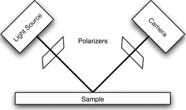

Another element of the optical equipment was a pair of polarizers, one in the illumination path and one in the detection path. Cross-polarizers were used to increase contrast. This is necessary because a higher percentage of the detected light is reflected from the surface of the phantom or blood vessel than from the particles flowing inside. Using polarized light makes it possible to enhance the signal from the underlying moving particles.

2.3.

Computer Simulations

Simulations were performed to evaluate the STICS analysis method described here for flow measurement. In these simulations, particles were represented as uniform disks moving in two dimensions. Fluid velocity was assumed to be constant throughout the observation volume (i.e., boundary effects were ignored) and was modeled as a displacement in the $x$ direction at each time-step of the simulation. Diffusion was included in this model as pseudo-random displacements in the $x$ and $y$ directions. This pseudo-random displacement was generated from a normal distribution with a mean of zero and a standard deviation of $\sigma ={\left(2D\tau \right)}^{1∕2}$ where $D$ is the diffusion coefficient in ${\text{pixels}}^2∕\text{frame}$ , and $\tau$ is the frame time. Simulations were performed both in ideal conditions and with both shot noise and constant background. All simulations were performed using MATLAB version 7.3.0.267 (R2006b) (MATLAB, Mathworks, Natick, Massachusetts).

The values of the parameters used in these simulations expressed in terms of pixels are as follows: Each simulated image was $256\text{pixels}$ by $256\text{pixels}$ , and the subregion analyzed was $64\text{pixels}$ by $64\text{pixels}$ . The radius of the simulated particles was $2\text{pixels}$ , but $1\text{pixels}$ gives similar results. The diffusion coefficient was $0.1{\text{pixels}}^2∕\text{frame}$ . The direction of flow was in the positive $x$ direction. The velocity of the particles was varied from $0\text{to}15\text{pixels}∕\text{frame}$ . These values can be considered to model data acquired in the manner presented in this article. The analyzed area is the same size for both simulated and actual data.

3.1.

Basic Theory

The challenge in measuring flow by intensity fluctuations is that these fluctuations are combined with other, large, irrelevant signals—namely, stationary objects, as illustrated in Fig. 2, and camera noise. This is why the flow rate is not immediately obvious when looking at a series of images and why statistical analysis methods must be employed. Specifically, we use spatiotemporal image correlation analysis (STICS). The technique presented here is a modified version of the STICS analysis developed by Hebert ¹¹ In this analysis, the signal from stationary objects is removed first, through subtraction of the average image. The camera noise is removed through correlation techniques. Camera noise, in our system, does not correlate spatially or temporally and therefore is not present in the correlation results.

Fig. 2

Physical source of optical signals (left) and images containing those signals (right). The optical signal from moving blood cells (a) is obscured by the signal from stationary objects such as the blood vessel wall (b) and camera noise (c). Figure is not drawn to scale.

Subtracting the temporal average of all images from each image eliminates the signal from any stationary objects in the field; otherwise, the correlation from stationary objects overwhelms the correlation signal from the moving object we are interested in. Subtraction of the average image has the consequence of changing the average intensity of each frame. This will in turn change the amplitude of the correlation. This method of removing stationary components is different from the low-pass filtering method used by Hebert.

The STICS calculation is defined in Eq. 1 ¹¹:

STICS is based on spatial correlations. The spatial cross-correlation function provides a method of mathematically evaluating the similarity between images. It is highest in value at spatial shifts ( $\xi$ and $\psi$ ) for which the second image $\left[i_a(x,y)\right]$ is similar in intensity to the first $\left[i_b(x,y)\right]$ . That is, it has a high value when the intensity of image $a$ at location $(x,y)$ is similar to the intensity of image $b$ at location $(x+\xi ,y+\psi )$ . A useful representation of a spatial correlation function, which is used here, is a 2-D plot in which the axes are $\xi$ and $\Psi$ , and the magnitude of the function is represented with a color scale.

The spatial cross-correlation function is particularly useful for extracting information about flow because there is a high degree of similarity between sequential images of flowing particles, and spatial cross-correlation analysis responds to this. Each particle in one image moves to a new location in the next image, and so on. The particle appears at a greater spatial shift in each successive image. This means that each image is essentially a shifted version of the earlier images. The displacement caused by flow will be approximately the same for each particle, since flow moves all particles in the same direction at the same rate. Therefore, for $G$ calculated between two successive images of flowing particles, there will be a peak in the spatial correlation function at a spatial shift equal to the displacement caused by flow.

In STICS analysis, the cross correlation is calculated between all pairs of images with a fixed time shift $\left(\Delta T\right)$ between them. For example, at $\Delta T=2$ , frame 1 is correlated with frame 3, frame 2 with frame 4, frame 3 with frame 5, etc. These cross correlations are then averaged. STICS can be calculated at more than one time shift ( $\Delta T=0$ , $\Delta T=1$ , $\Delta T=2$ , etc.). Larger shifts should give the most accurate measurement of flow, since they include position at longer time delays; however, this is limited by diffusion and particles that move out of frame. We calculate STICS at multiple time shifts to obtain the maximum amount of temporal information and to improve the accuracy of the flow rate obtained through fitting the data as described here.

3.2.

Extracting Velocity from STICS

The peak value of the STICS correlation plot is shifted from the center in the direction of flow by an amount that relates to the speed at which the particles are traveling. Average velocity can be extracted as described in Eq. 2:

More precise numerical information is extracted from STICS analysis by fitting the experimental STICS plot to a 2-D Gaussian [Eq. 3]:

3.3.

Mapping Flow

In the data presented here, STICS analysis and global data fitting was done in regions $32\text{pixels}$ by $32\text{pixels}$ that overlap by $16\text{pixels}$ . Using a small area improves data processing speed. Additionally, it makes it possible to map flow by improving resolution. In the experimental data presented here, each 32-by- $32\text{pixel}$ analysis region corresponds to an area $0.32\mathrm{mm}$ by $0.32\mathrm{mm}$ , meaning that the resolution of such a map is less than $1\mathrm{mm}$ . The results of flow mapping are displayed using arrows to represent the velocity. One arrow is placed in the center of each region of analysis. The length of the arrow corresponds to the magnitude of the velocity as calculated in Eqs. 2, 4. The direction of the arrow corresponds to the direction of flow as determined using Eq. 5. Arrows are plotted for each region of analysis in which the amplitude of the STICS peak is above a threshold value.

3.4.

Distinguishing Laminar and Turbulent Flow

Laminar and turbulent flow have distinct STICS plots when the region of analysis is large enough relative to the scale of the flow pattern. Laminar flow is characterized by velocities that vary spatially in magnitude but not in direction. This results in an STICS peak that is elongated in the direction of flow. Turbulent flow has a velocity pattern that varies both spatially and temporally in magnitude and direction. Turbulent flow often contains circulating regions or eddies. This type of flow causes the STICS peak to become wider as $\Delta T$ increases until it stabilizes at a maximum width. The peak will also move in the direction of the overall flow.

4.1.

Computer Simulations

The results presented here make clear that fluid velocity can be measured using STICS analysis. Representative results of the computer simulations can be seen in Fig. 3 . STICS analysis of simulated data with a constant flow rate is presented at two different STICS shifts. The STICS plot on the left where the STICS shift is zero $(T=0)$ does not provide any information about flow, since it is the average of the spatial autocorrelation of each frame (the cross correlation of a frame with itself), and the location of the STICS peak does not change regardless of the velocity. The size of the STICS peak at $T=0$ is related to the size of the particles at small particle velocities.

Fig. 3

STICS analysis of simulated data plotted at two STICS shifts (and frames). The simulated data has a velocity of $10\text{pixels}∕\text{frame}$ , and this is reflected in the STICS peak shift of $20\text{pixels}$ .

The velocity can be extracted from the location of the peak at different $\Delta T$ using the simulation parameters and Eqs. 2, 3. A plot of this extracted velocity is shown in Fig. 4 . The method is accurate and requires only calibration to determine the size of the image. This can be accomplished by placing a ruler in the field of view.

Fig. 4

Measured velocity versus simulated velocity. Velocity was calculated as described in Eq. 2.

4.2.

Blood Flow Phantoms

In Fig. 5, we show the peak of the STICS plot at $\Delta T=5$ for two flow rates. At a flow rate of 0, the STICS peak is located at the origin, and at a nonzero flow rate, the location of the STICS peak moves farther from the center of the plot. Fluid velocity can be extracted from STICS analysis using the method described earlier. Figure 6 shows the extracted fluid velocity plotted versus the applied flow rate. The correlation coefficient between the two is $R=0.94$ .

Fig. 5

STICS results for a shift of five frames and at two flow rates. As the flow rate increases, the location of the STICS peak shifts in the direction of flow.

Fig. 6

Velocity measured using NIR-STICS versus the nominal flow rate. The flow rate reported by the syringe pump was faster than the actual flow rate by a factor of approximately 5 due to impedance in the microfluidic system. The results of five trials at each flow rate are plotted here.

4.3.

Flow Mapping

The most important feature demonstrated by our experiments is that STICS can be used to map flow in multiple channels over an area. In Fig. 7, STICS analysis was used to map flow in two different channels simultaneously with different flow rates, as described in Sec. 3.3. In the top channel, the flow rate is faster, and this is reflected in the longer arrows.

Fig. 7

STICS analysis for two different microchannels in the same image with the calculated flow rate represented as arrows. Analysis was performed in regions $32\text{pixels}$ by $32\text{pixels}$ that overlapped by $16\text{pixels}$ . Arrows represent the direction and magnitude of the velocity. The average velocity is $3.9\mathrm{mm}∕\mathrm{s}$ in the top channel and $2.6\mathrm{mm}∕\mathrm{s}$ in the bottom channel.

4.4.

Distinguishing Laminar and Turbulent Flow

An additional and potentially important implication of the STICS methods is that NIR-STICS could distinguish between turbulent and laminar flow, as discussed in Sec. 2. The most straightforward way this can be accomplished is through the mapping procedure described earlier. Complex flow patterns on a certain scale within a channel will be reflected in the range of velocities found over the area mapped. This type of flow mapping is accessible by other techniques, including Doppler.⁷ There is, however, a more subtle and unique way that STICS can distinguish between laminar and turbulent flow: the shape of the STICS peak is determined by the flow pattern within the region of analysis. Figure 8 contains an example of laminar and turbulent flow analyzed with STICS. The turbulent flow was obtained by partially obstructing the flow channel. The laminar flow plot is elongated in the direction of flow, and it is asymmetrical. This reflects particles moving at varying speeds but overall in the same direction within the region of analysis. The STICS plot for the turbulent flow is round and more symmetrical. This is due to particles moving in many directions locally (an eddy) but in one direction overall.

Fig. 8

STICS analysis of laminar and turbulent flow, both at $\Delta T=2$ . Laminar flow is reflected in an elongated, asymmetrical STICS peak. The STICS peak for turbulent flow broadens in all directions. The white circles are included to identify the region of interest and are not computationally significant.

5.1.

Instrumentation Considerations

In the STICS technique, measurements must be made with a frame rate and maximum $\Delta T$ that are appropriate for the velocity being measured. If the frame rate is too slow, the particles will move out of the image before a second image is acquired, and it will be impossible to recover the velocity. The need for a fast frame rate has to be weighed against taking measurements over a large area, since using larger frame sizes will slow the frame rate. The exposure time also needs to be large enough to obtain a sufficient signal-to-noise ratio for the level of illumination. Increasing the exposure time will also slow the frame rate. The frame rate and maximum $\Delta T$ must also be appropriate for the velocity being measured. At frame rates that are too slow and $\Delta T$ values that are too large for the velocity, the STICS peak will “wrap around” to the opposite side of the STICS plot, and flow will appear to be in the opposite direction. For example, at a velocity corresponding to $10\text{pixels}$ /frame in the positive $x$ direction and a region of analysis of $32\text{pixels}$ by $32\text{pixels}$ , the STICS calculation at $\Delta T=1$ will be accurate with the peak located at $\xi =10$ . However, when $\Delta T=2$ , the STICS peak will be located at $\xi =-13$ . This problem can be identified by calculating STICS for several values of $\Delta T$ and observing whether the apparent direction of flow varies.

It is important to realize that the key feature of the STICS plot is the peak. The background may also have features, as can be seen in Figs. 3, 5, 8, and it is rarely equal to zero at every point, but the amplitude of these features is several times less than the amplitude of the peak due to the moving particles. In Fig. 5, for example, the amplitude of the peak is $9\times {10}^{-5}$ , while the highest point outside the peak is $3\times {10}^{-5}$ . There is no pattern observed between data sets for these features, and increasing the number of frames acquired further decreases the amplitude of the surrounding peaks.

STICS flow maps can be created with varying resolutions depending on the size of the region of analysis. Smaller regions of analysis give greater resolution and are faster to calculate but are also more sensitive to noise. Large regions of analysis average the flow rate over a larger area and are appropriate when the average flow through a region is needed.

The experiments presented here were all performed on phantom systems that were designed to closely mimic physiological systems. The channels were the same size as the blood vessels of interest, flow rates were in the correct range, and the scattering particles were similar in size to blood cells. However, there were limitations to this phantom system. One important limitation was that the material used to create the phantoms was transparent, while actual tissue scatters lights. Actual tissue would add stationary objects to the measurement that the background subtraction step would remove. Phantoms were used to control the experimental parameters more precisely and to accurately test the performance of the technique.

5.2.

Medical Applications of NIR-STICS

NIR-STICS is a robust statistical technique and could be adapted to map blood flow during surgery. The technique relies on optical signals. It is effective even when individual blood cells cannot be resolved by the microscope. The STICS analysis extracts the rate of flow from optical fluctuations caused by individual particles.

The range of velocities accessible to NIR-STICS is limited only by the frame rate of the camera and the size of the region being analyzed, which is in turn dependent on the magnification and the desired resolution of the flow map. With the parameters described here, fluid velocities ranging from less than $1\mathrm{mm}\text{per}\text{second}\text{to}25\mathrm{mm}\text{per}\text{second}$ can be measured. Blood flow in the human body typically ranges from millimeters per second in the capillaries up to a meter per second in large arteries.^{15, 16} Faster frame rates and larger frame sizes would allow measurement of faster velocities. Slower velocities could be measured by acquiring data over a longer time frame. NIR-STICS in its present implementation does not encompass the entire range of blood flow rates in the human body but does provide a way to measure slower velocities that are difficult to measure with Doppler techniques. Moreover, with the parameters used here, NIR-STICS measurements can be performed in near-real time.

In addition to accessing a range of fluid velocities, NIR-STICS can be adapted for blood vessels of different sizes. The resolution of the image analyzed through STICS is dependent only on the magnification used to create the image. Blood vessels as small as capillaries will be accessible to NIR-STICS. Flow through any blood vessel less than approximately half a centimeter in diameter can be measured with this technique. Larger blood vessels will have higher fluid velocities and thicker vessel walls and are less suited to NIR-STICS measurements. Again, NIR-STICS makes previously difficult measurements possible through its effectiveness on smaller blood vessels.

Furthermore, NIR-STICS is suited to measuring blood flow because it is insensitive to small temporal variations in flow. This means that pulsatile variability will not diminish the accuracy of NIR-STICS measurements. Even in the case of blood cells moving through capillaries slowly, one at a time, NIR-STICS can still provide an accurate measurement of the average velocity.

NIR-STICS could be used as the basis of a device to measure blood flow in exposed blood vessels during surgery. Such an instrument would be an improvement over existing technology in that it is noncontact, does not require the use of contrast agents, and can create a map of flow over a relatively large area. Additionally, the optics are such that they can be easily incorporated into existing surgical microscopes.

In addition to measuring fluid velocity, NIR-STICS as applied in the reflection mode should be able to determine other information such as the concentration of moving particles in the observation volume. This could also have medical applications, as the number of blood cells is directly related to the rate at which oxygen reaches tissue.

5.3.

Distinguishing Laminar and Turbulent Flow

NIR-STICS also has the potential to address medical issues related to turbulent blood flow. Turbulence can be caused by vascular anomalies, including aneurysms, plaques, and diseased heart valves. Identifying turbulent flow and understanding its underlying causes is important to treat these conditions. The ability to distinguish between laminar and turbulent flow is an inherent property of NIR-STICS. This makes NIR-STICS a potentially valuable tool for examining blood flow in large blood vessels as well as the smalls blood vessels that are the focus of the experiments presented here.

5.4.

Comparison to Speckle

It is important to acknowledge the differences and similarities between NIR-STICS and laser speckle. While it remains to be seen what the true strengths and weaknesses of laser speckle are, it is clear that NIR-STICS will have advantages in that it can determine the direction of flow and it can be used to map flow over an area. A single point speckle measurement takes several seconds. This can make scanning, and therefore mapping, impractical. An additional complication with speckle is that it requires a mathematical model to extract the flow rate from the rate of fluctuation. In STICS analysis, the average displacement between frames can be determined directly from the location of the STICS peak, whereas in speckle techniques, assumptions must be made to relate the time scale of speckle fluctuations to the rate of flow.