
|
|
1.IntroductionNoninvasive optical 3-D imaging in biological tissues has been studied for decades because of its high sensitivity and specificity.1, 2 Unfortunately, optical techniques suffer from low spatial resolutions when imaging deep tissue due to the high light scattering of tissue.2 To overcome this drawback, ultrasound-modulated optical tomography (UOT) has been developed.3, 4, 5, 6, 7, 8, 9, 10, 11, 12, 13, 14, 15, 16, 17 When UOT maintains high ultrasonic spatial resolutions, it provides tissue optical information.3,4,5,6,7,8,9,10,11,12,13,14,15,16,17 However, since modulated photons coming from the ultrasound focal zone are usually a very small portion of the total unmodulated photons from both the focal zone and the entire tissue, UOT has low signal-to-noise ratio (SNR) or modulation depth (defined as the ratio of modulated photons to unmodulated photons received by a detector), which prevents using this promising technique in clinical applications.10,11,12,13,14,15,16,17 Recently, significant improvements in SNR have been achieved based on different detection schemes,3,4,5,6,7,8,12 which enables UOT use for studying living systems. Since fluorescence provides unique tissue physiological information and is sensitive to tissue microenvironments,18 such as tissue pH value, gas, or ion concentrations, developing ultrasound-modulated fluorescence tomography (UFT) is also interesting. Recently, UFT has been proposed and demonstrated.9, 19, 20, 21, 22, 23, 24, 25, 26 Compared with UOT, UFT is even more challenging due to the incoherent property of fluorescence. Also, modulation mechanisms may be different from those of UOT.26 Thus, the techniques developed for improving UOT SNR may not be applicable to UFT. To improve SNR or modulation depth in UFT, increasing modulation efficiency in the focal zone and reducing background emission are considered as two important directions. By significantly quenching background fluorophores and activating fluorophores in the focal zone (especially based on fluorescence resonance energy transfer, or FRET), the modulation depth may be dramatically improved.20, 24, 26 In fact, Chen have reported a “switch-like” relationship between fluorescence lifetime of 5(6)-carboxyfluorescein (6CF) and its concentration in liposomes27 (see Fig. 6 in Ref. 27). Fluorescence lifetime of 6CF maintains a constant ( , its natural lifetime) until the concentration reaches . Lifetime rapidly reduces to , when concentration is increased from . This precipitous change in fluorescence lifetime was found due to FRET from excited 6CF molecules to nonfluorescent 6CF dimmers.27, 28 (Quantum yield is supposed to follow a similar relationship when FRET is the quenching mechanism.) Importantly, such a switch-like relationship implies that one may define three states for fluorophores (6CF) based on concentrations (C): “on” , “transition” , and “off” states. Therefore, if one can initially control fluorophores at the off state and ultrasonically switch on only those fluorophores in the focal zone by dramatically changing the concentration (essentially changing the distance between a fluorescent molecule and its quencher: F-Q distance), the background fluorescence can be reduced and the modulation efficiency in the focal zone can be improved. The challenge becomes how to efficiently control the fluorophore concentration or F-Q distance. Microbubbles (usually used as contrast in ultrasound imaging) compressed or expanded by an ultrasonic wave may be used to change the surface concentration of fluorophores labeled on the bubbles or F-Q distance.20, 24, 26 It has been shown that a negative ultrasound pulse with a modest pressure can easily expand the bubbles’ radius several times larger without fragmentation.29 Recently, a similar idea of labeling microbubbles with fluorophores and quenchers (F-Q microbubbles) has been proposed.20, 24, 26 Although the principle of combining microbubbles with the FRET quenching effect is straightforward, it will be valuable if a model can be given and used for predicting the possible improvements in modulation depth due to adopting F-Q microbubbles. Also, since currently there are no experimental data available in the literature, theoretical studies become more important because they may provide a guideline for designing experiments and potentially provide valuable implications for experimentalists. Therefore, in this study, the modulation depth is quantified by solving a governing equation of microbubble oscillation in ultrasonic pressure field (the modified Herring equation),29 a two-energy-level rate equation describing the excitation of fluorophore in the optical field,30, 31 and a diffusion equation characterizing the propagation of highly scattered photons in tissue.2, 32 Two possible imaging modes (fluorescence intensity and fluorescence lifetime) are investigated based on three different illumination modes of the excitation light: continuous wave (direct current, or DC), radio frequency–modulated excitation light (frequency domain, or FD), and ultra-short pulse excitation light (time domain, or TD). Modulation depths are quantified for the three illumination modes. Strategies for improving the modulation depth are discussed. 2.Theoretical Models2.1.Nonlinear Oscillation of MicrobubblesMicrobubbles can oscillate nonlinearly in a very low ultrasonic pressure field. The oscillation of a bubble’s radius can be obtained by solving the following modified Herring equation:29 The modified Herring equation provides more accurate results than the Rayleigh-Plesset equation when the expansion ratio in the radius of a microbubble is greater than 2. (Expansion ratio is defined as the ratio of the instantaneous bubble radius to the initial radius.29) Notation in Eq. 1 is given in Table 1 (the numbers or formulas following each notation are used for numerical calculation in this study), and the details about Eq. 1 have been discussed in Ref. 29. Numerous studies have demonstrated that a microbubble can be easily expanded more than 10 times larger than its initial size with appropriate peak rarefactional pressure (PRP) in large vessels .33, 34, 35 Although studies have shown that the small vessel wall may limit the expansion ratio of a microbubble,33, 34, 36, 37, 38, 39 approximate three times expansion (without bubble fragmentation) for a microbubble with a diameter of has been observed in a small vessel with a diameter of in cecum tissue under PRP ultrasound insonation.34 Based on these studies, the expansion ratio in this study is limited below three. For simplicity, no interactions between bubbles and vessel wall are considered in this study. Therefore, PRP can expand a microbubble ( in diameter) three times based on Eq. 1, and the parameters used in the calculation are listed in Table 1. For simplicity, the driving pressure is assumed as a sinusoidal pressure wave, , and the window function is for selecting the number of cycles of the pressure wave. In this study, only one cycle is used.Table 1Notation of acoustic parameters (microbubble, surrounding medium, and ultrasound).
2.2.Photon Propagation in Tissue in Three Modes: DC, FD, and TDPhoton propagation in tissue has been well modeled as a diffusion equation based on certain assumptions.31, 32 Green’s function method is usually used to solve the diffusion equation for fluence of excitation and emission photons.31, 32 Generally, three types of illumination modes of excitation light have been adopted in the literature: DC, FD, and TD modes.31, 32 The illumination intensity of the excitation light is a constant for the DC mode, a sinusoidal function of time (with radio frequency ) for the FD mode, and an ultra-short pulse (in the order of picosecond) for the TD mode. Equation 2 is a solution to the diffusion equation and describes the spatial distribution and temporal change of the fluence of the excitation light in DC and FD modes:31, 40 where is the DC component of the fluence of the excitation light at position illuminated by a point source at position . is the amplitude of the fluence of the corresponding alternating current (AC) component. is the modulation frequency of the excitation light, is the time taken by the ultrasound pulse traveling from the medium surface to the upper edge of the ultrasound focal zone (see Fig. 1 ), and is the phase delay caused by the propagation of photon density wave from the point source to the position and equal to . For a semi-infinite medium with an extrapolated boundary condition, and can be expressed as the following equations:31, 40 where , , , . and are the strengths of the DC and AC components of the light source, respectively, with unit of photons/second. is the distance between the source and the position , and is the distance between an image source and the position Refs. 31, 40. Similarly, for TD mode, the fluence can be expressed as follows:32 where relates to the pulse strength with unit of photons/second, and other parameters are defined in Table 2 and Ref. 32. in the subscript represents that the incident light pulse is launched only at the position .Fig. 1The acoustic and optical setup in simulation: S and D represent the excitation light source and the detector. The solid arrow indicates the propagation of the diffused excitation photon from the source to a point in the focal zone, and the dashed arrow represents the propagation of the emitted fluorescence photon from that point to the detector. The two dotted curves represent ultrasound waves, and the cylinder represents the ultrasound focal zone. A and B indicate the radius and the length of the focal zone. represents the distance between the source and the detector. 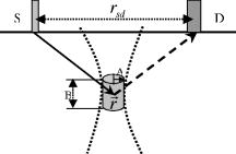 Table 2Notation of optical parameters (medium, fluorophore, and light source).
2.3.Excitation and Quenching of Fluorescent Molecules on the MicrobubblesWhen photons reach position , fluorescent molecules on the bubbles absorb photons and are excited from ground states to high-energy-level states. The number of excited fluorescent molecules is determined by the following rate equation when a two-energy-level model is adopted:30, 31, 40 is the molar concentration of fluorescent molecules at excited states, is the total decay rate including both radiative and nonradiative decay , is the molar extinction coefficient at the wavelength of the excitation light, is the fluence of the excitation light at position and time , and is the total molar concentration of fluorescent molecules at position . Inserting Eq. 2 or 5 into Eq. 6, can be solved as a function of position and time , and the emission strength of the fluorescent molecules at the position and time can be calculated from the following equation:30, 31, 40The corresponding results for DC, FD, and TD are solved as follows: Equations 8, 9, 10 represent the emission strengths in DC, FD, and TD modes, respectively. ⊗ in Eq. 10 represents convolution. In the derivations of the three equations, an initial condition, , was used. The exponential decay terms in Eqs. 8, 9 represent the transient solutions, and the other terms indicate the steady-state solutions. Since the lifetime is usually on the order of nanoseconds, the transient solution may be ignorable. However, for Eq. 10, the exponential decay term has to be convolved with the pulse of the excitation light. In this study, the transient solution in Eq. 8 is ignored because only the steady-state solution is interesting for DC mode. Although the transient solution in Eq. 9 is considered in our following numerical calculation, its contribution may be small. Therefore, a simplified solution is also provided on the last line of Eq. 9 by ignoring the transient solution and combing the last two terms. The phase angle in Eq. 9 is expressed as:The fluorescence fluence at the detector position can be obtained: are Green’s functions at emission wavelength in DC, FD, and TD modes and can be obtained from Eqs. 3, 4, 5 by dropping the source strength related terms ( , , and ), respectively, and changing all the excitation light (“ex”) related terms to the emission light (“fl”) related terms. is the volumetric region of the ultrasound focal zone. ⊗ represents convolution.Based on FRET theory,28, 30 the quantum yield and lifetime are a function of the distance between the fluorophore and its quencher, and therefore a function of the bubble’s radius and can be expressed as follows: In the derivation of Eqs. 13, 14, the microbubble is assumed as a sphere with radius , and both fluorescent molecules and quenchers are uniformly distributed on the bubble surface. The total number of fluorescent molecules and quenchers is ; therefore, the distance between any two adjacent molecules can be approximated as . is the Förster distance, which is a characteristic parameter of the fluorophore quencher. and represent the quantum yield and lifetime at the absence of FRET quenching, respectively—for example, when the bubble is opened so large that FRET quenching is ignorable. When there are no other quenching mechanisms, and should be considered as the natural quantum yield and natural lifetime. However, if other quenching mechanisms exist at a specific position, and will reflect the quantum yield and lifetime affected by the local environment, which can be used to detect tissue physiological properties. 2.4.Summary of the Models and Methods of Numerical CalculationSince the bubble’s radius oscillates with ultrasound pressure, which can be solved from Eq. 1, the quantum yield and lifetime become a function of time, which is solved by inserting the solution to Eq. 1 into Eqs. 13, 14. The resultant quantum yield and lifetime (as a function of time) are inserted into Eqs. 8, 9, 10, respectively, and the local emission strength, , can be calculated for the three excitation modes. Eventually, based on and the Green’s function , the fluorescence fluence at the detector position can be obtained from Eq. 12. Since Eq. 1 is a second-order nonlinear differential equation, the equation is put into a dimensionless form.29 Two initial conditions are and at time . is the initial bubble radius. The ordinary differential equation solver in MATLAB is used to solve the nondimensional form of Eq. 1. Other numerical calculation is implemented using MATLAB, and all parameters used in this study are listed in Tables 1, 2. 3.Results and DiscussionsFigure 1 shows the schematic used in this study. The and represent the laser source and detector positions, respectively. indicates the distance between the source and the detector. The two dotted lines represent the focused ultrasound wave, and the cylindrical region shows the ultrasound focal zone. and indicate the radius and length of the focal zone. The modulation of microbubbles is considered only in this focal zone because of its much higher pressure than that in the surrounding region. In practice, two crossed ultrasound beams may be used to increase the pressure difference between the focal zone and the surrounding region. In this study, the time is initiated when the ultrasound pulse reaches the upper edge of the focal zone. This is implemented in Eqs. 8, 9, 10, 11, 12, 13, 14. 3.1.Microbubble OscillationFigure 2 plots the expansion ratio of a microbubble as a function of time driven by a sinusoidal ultrasonic pulse. For comparison, the driving pressure pulse is normalized by its amplitude and up-shifted by adding 1. It is clear that the bubble is quickly compressed at the positive half-cycle of the pressure pulse and slowly expanded up to 3 times larger in radius in the negative half-cycle of the pressure pulse. The rest of the oscillation is caused by free oscillation of the microbubble. The first important implication from this result is that the radius of the microbubble can be easily expanded 3 times greater than its initial radius, and therefore the distance between a fluorescent molecule and its quencher can increase 3 times relative to the initial distance. The surface concentration of fluorophores may be reduced 9 times. From FRET theory,28, 30 the quenching efficiency will be significantly decreased because of the sixth power relationship between the molecule distance and the quenching efficiency [see Eqs. 13, 14]. Consequently, strong fluorescence emission should be generated during the bubble expansion period due to the low quenching efficiency. Thus, the ultrasonic pulse serves as a tool to open a time period during which the fluorophores are switched on and emit strong fluorescence, which may provide considerably strong signals from the focal zone compared with the unwanted fluorescence emission from those bubbles in the surrounding regions where high quenching efficiency exists. Fig. 2Expansion ratio of a microbubble (solid line) driven by a single sinusoidal ultrasound pulse (dashed line) as a function of time. For comparing two curves, the driving ultrasound pulse is normalized by its peak value plus one. 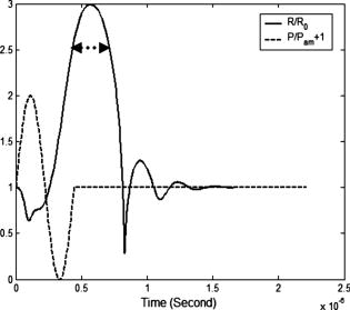 The second important implication from Fig. 2 is that the time duration is about when the bubble radius is expanded 2.5 times greater than its initial radius (indicated by the dotted arrows). This result means that even a single microbubble driven by a single ultrasonic pulse can provide enough time window for measuring fluorophore lifetime because the lifetime of the fluorophore is usually in the order of nanoseconds. By using FD and TD excitation modes, the lifetime of the fluorophore may be measured during that period. This will be further discussed later. Also, the bubble oscillation is obviously delayed compared with the driving pressure pulse. These results for bubble oscillation are in good agreement with those reported in the literature and have been verified by experimental measurements based on ultra-fast photography.29, 41 3.2.Intensity Imaging ModeEquations 8, 9, 10 show that the measured fluorescence fluence is directly proportional to the fluorophore concentration in the focal zone. Therefore, it is straightforward to image the fluorophore concentration distribution (also the bubble distribution) in the tissue based on the fluorescence signal strength. This is a typical imaging mode in UOT and UFT because the concentration distribution may correlate with some tissue physiological status, such as tumor angiogenesis and blood perfusion. Figure 3 provides the simulated results about the fluorescence fluence as a function of time excited by the three different illumination modes, DC [Fig. 3a], FD [Fig. 3b], and TD [Fig. 3c], at the point source position S, generated from the ultrasound focal zone, and received at the detector position D (see Fig. 1 for the geometry). In Figs. 3a, 3b, 3c, the solid lines show the fluorescence fluence generated from the ultrasound focal zone. The depth of the focal zone (from the surface of the medium to the center of the focal zone) is and the source-detector separation is indicated on the figure. The fluorescence fluence is considerably low before , which corresponds to the bubble-compressing period and is in agreement with the result showing in Fig. 2. From to the time at which the fluence reaches the maximum (indicated by arrows), the fluence rapidly increases and corresponds to the significant expanding of the bubble in Fig. 2. However, the peak positions in Fig. 3 are not exactly the same as the peak position in Fig. 2. This is because the fluorescence fluence in Fig. 3 is calculated from the integral over the whole focal zone, instead of from a single bubble, as in Fig. 2. Fig. 3Fluorescence fluence at the position of the detector as a function of time for three different illumination modes of the excitation light: (a) DC, (b) FD, and (c) TD. The solid lines in the three figures represent the fluence generated from the focal zone. The dotted line in (a) and (b) represents the fluence from the background and is divided by 20 for plotting. The time zero in the three figures means the time at which the wavefront of the ultrasound pulse reaches the upper edge of the focal zone. The depth of the focal zone for all three figures is , and the source-detector separation is also listed on each figure. The insets in (b) and (c) show the enlarged portions of the peak regions of the original figures, which are indicated by arrows in the figures. 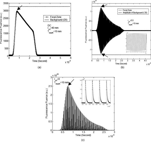 The third period between the peak position to is caused by the propagation of ultrasound pulse in the focal zone, and the gradual decay of the fluorescence fluence during this period corresponds to the decrease of the fluence of the excitation light with the increase of the depth of the ultrasound pulse in the focal zone. From , the fluorescence fluence decays even faster. This corresponds to the period that the ultrasound pulse exits the focal zone, and the decay rate may relate to the fast recovery of the expanded bubble. After this period, the ultrasound pulse propagates out of the focal zone, and very weak signal can still observed, which is generated due to the non-100% quenching of the fluorophore on the bubbles. For simplicity, the decay of ultrasound in the focal zone is ignored. However, it is straightforward to consider its effect by adding a decay coefficient when calculating the propagation of the ultrasound pulse in the focal zone. The most interesting period is in the peak region indicated by the arrows. The insets in Figs. 3b and 3c show the enlarged figures when the fluence reaches the peak values. It can be seen that the fluorescence fluence is modulated with high frequency ( in this study) in Fig. 3b for FD mode or pulsed at high repetition rate ( period between two light pulses) in Fig. 3c for TD mode. To investigate how strong the ultrasound tagged photons are in comparison with the untagged photons from the background medium, fluorescence fluence generated from the surrounding region of the ultrasound focal zone is also calculated based on similar equations and source-detector setup, except for the following differences: (1) the integral volume is over the whole semi-infinite medium; and (2) bubble radius is assumed as a constant, the initial bubble radius , during the entire time period, and therefore, the quenched quantum yield and lifetime are constants. Although the quantum yield and lifetime of the fluorophore in the background medium is quite small due to the high quenching efficiency, the large integral volume and the strong excitation fluence around the light source may lead to strong background signal, which should be considered as noise relative to the tagged photons from the focal zone. The dotted line in Fig. 3a indicates the fluorescence fluence generated from the background region, and the dotted lines in Fig. 3b show the positive and negative amplitudes of the modulated fluorescence fluence generated from the background. To make the background signals visually comparable with the tagged fluence from the focal zone, the background signal in both Fig. 3a and 3b has been divided by a factor of 20. By defining the ratio of the maximum of the ultrasound tagged fluorescence fluence to the fluorescence fluence generated from the background medium as the perturbation or the modulation depth, a quantitative study about the percentage of the perturbation as a function of the depth of ultrasound focal zone is shown in Fig. 4 . Three sets of data are presented in the figure, and each is circled with an ellipse to indicate it as a group. The three solid lines with squares represent the results with zero source-detector separation for the three illumination modes: DC—open squares, FD—solid squares, and TD—small solid squares. The three dashed lines with circles show the results with source-detector separation for the three illumination modes: DC—open circles, FD—solid circles, and TD—small solid circles. The three dotted lines with up-triangles show the results with source-detector separation for the three illumination modes: DC—open up-triangles, FD—solid up-triangles, and TD—small solid up-triangles. Fig. 4Percentage of perturbation (or modulation depth defined as the ratio of the peak fluence generated from the ultrasound focal zone to that from the background medium) as a function of the depth of the focal zone for the three illumination modes with different source-detector separations: (up-triangles), (circles), and (squares).  Several important implications can be obtained from Fig. 4. First, compared with the modulation depth in conventional UFT, the modulation depth has been significantly improved. As an example, under the similar ultrasonic and optical conditions, the modulation depth of UFT (based on the mechanism of fluorophore concentration modulation) is (Ref. 26). However, for the fluorophore-labeled microbubble system, the modulation depth is greater than 3% when the ultrasound wave is focused at a depth of (except the DC mode with zero source-detector separation). The perturbation is even when the focal zone is very close to the boundary. This significant improvement attributes to the high compressibility of the microbubble, high sensitivity of fluorphore quantum yield to the bubble size change, and extremely low quantum yield and short lifetime of fluorophore in the background medium. In practice, the modulation depth can be further improved when considering the fact that the skin tissue close to the laser source usually has fewer blood vessels than tumor tissue and therefore fewer microbubbles around the source location that can significantly reduce the background signal. Second, as the focus depth increases, the perturbation or the modulation depth reduces rapidly. This is because both the excitation fluence and the emission fluence decay fast with the increase of the depth of the ultrasound focus [see Eqs. 3, 4, 5, 12]. The longer source-detector separations provide the larger perturbations in the deep region, and the shorter separations show the larger perturbations in the shallow region. Therefore, to image deep tissue, large separations should be adopted. Note that for the case with zero separation, the calculated perturbation may not correctly reflect the truth because the diffusion model of photon propagation provides results with low accuracy in the calculation of the background signal. However, the calculation of the tagged fluorescence fluence in Fig. 4 is less affected by the diffusion approximation because the depth of the focal zone is nonzero. For 20- and separations, the perturbation in DC illumination mode is close to that in FD mode, and both are smaller than that in TD mode. The difference may be caused by a fact that the peak value of an emission pulse, instead of the total energy of the pulse (which is equivalent to the strength in DC mode), is used to calculate the tagged fluorescence fluence and the perturbation. Third, since the background emission can be measured before firing the ultrasound pulse, the tagged fluorescence photons can be extracted by subtracting the background signal from the total measured signal that includes both background signal and the tagged signal. Therefore, the tagged fluorescence may be an indicator of the local fluorophore concentration (or the bubble concentration). Thus it is possible to perform 3-D imaging of fluorophore concentration based on a 3-D scanning of the measurement system. Fourth, when the depth of the focal zone is greater than , the modulation depth is small. TD illumination mode may be a good option to obtain large modulation depth by temporally separating tagged photons from untagged photons (see Sec. 3.3.2). 3.3.Lifetime Imaging ModeLifetime imaging is particularly interesting in recent years because the lifetime of the fluorophore is very sensitive to tissue microenvironments. Furthermore, lifetime imaging can easily avoid most error sources due to unwanted or unknown intensity fluctuations, such as unknown fluctuations of excitation light caused by tissue optical heterogeneities and unexpected fluorophore or microbubble concentration fluctuations in blood vessels. Generally, both FD and TD techniques can be used to measure fluorophore lifetime in either microscopic or tomographic imaging modality.42, 43, 44 In the FD technique, phase delay is used to quantify fluorophore lifetime. In the TD technique, lifetime is quantified by directly measuring the delay of the emission pulse relative to the incident pulse of the excitation light. These two techniques have been investigated intensively in the literature.30, 42 As mentioned earlier, since the “transition” state of fluorophores is relatively narrow (which is due to the sixth power relationship between the FRET quenching efficiency and the F-Q distance),27, if one can completely switch the fluorophores from off to on state, the quenching caused by FRET will be completely disabled. The lifetime will be the natural lifetime of the fluorophore when no other quenchers exist. If other quenchers exist (such as oxygen), the fluorophore lifetime may mainly depend on these quenchers when FRET is completely disabled. Usually, the lifetime changes caused by local tissue microenvironments are relatively smaller in comparison with the lifetime change when fluorophores alternate between off and on states. Therefore, lifetime variations caused by non-FRET quenching may be viewed as perturbations of natural lifetime when fluorophores are completely at the on state. Equations. 13, 14 indicate that both the quantum yield (related to emission intensity) and the lifetime (related to phase delay or pulse delay) are a function of time during the bubble expansion period. By examining the phase delay in FD mode or pulse delay in TD mode when the emitted fluence reaches the peaks in Fig. 3, possible lifetime imaging may be developed. 3.3.1.Lifetime imaging in FD modeFigure 5a shows a single cycle of the emitted fluence as a function of time in FD mode around , which corresponds to the peak region in Fig. 3b. The source-detector separation is zero, and the depth of the ultrasound focal zone equals . To investigate the effects of lifetime on the fluence, varies from . The fluence from the background medium is also plotted as a reference. For comparison, each curve is normalized by its maximum. It can be seen that the wave of the fluence shifts toward the right side when increasing the lifetime . Figure 5b presents the quantified phase delay of each case relative to the background fluence. Phase delay increases from when increases from . Thus, a total of phase difference is obtained. This is a large phase shift compared with a sensitivity of phase measurement in heterodyne detection technique (depending on signal-to-noise ratio).30, 45, 46 Although diffusion approximation may cause an error in the calculation of background signal, this error does not affect the preceding analyses about the phase shifts because the background signal is used only for a reference and only the phase shifts between different lifetimes are of interest. In addition, in practice an external reference signal, instead of the background signal, with appropriate strength may be used as a reference signal.46. In FD mode, the tagged signal is mixed with the background signal because both of them oscillate with the same modulation frequency ( in this study). To distinguish the tagged signal, the background signal has to be measured separately and subtracted from the mixed signal. This will limit the system sensitivity because the strong background signal usually generates strong shot noise. Thus, the detection limit is determined by the shot noise. Fig. 5(a) A single cycle of normalized fluorescence fluence around the peak position in Fig. 3b, which is generated from the ultrasound focal zone and in FD mode. The lifetime is decreased from . The normalized fluence from the background medium with is also plotted for comparison. (The background fluence is almost independent of lifetime .) (b) Phase delay (degree) of the fluence in (a) relative to the background fluence as a function of lifetime . (c) A single pulse of the emitted fluorescence fluence around the peak position in Fig. 3c, which is generated from the ultrasound focal zone and in TD mode. The dotted line indicates the emitted fluorescence from the background medium with . The dashed line represents the sum between the fluence from the background medium (the dotted line) and the fluence from the ultrasound focal zone with (the solid line with asterisks). Lifetime with 3.5, 3, and are also plotted in the figure. The corresponding background fluence is not shown in the figure because it is almost the same as the dotted line.  3.3.2.Lifetime imaging in TD modeFigure 5c shows a single pulse of the emitted fluorescence fluence received by the detector around , which corresponds to the peak region in Fig. 3c. The source-detector separation is zero, and the depth of the focal zone is . (Other source-detector separations give similar results.) The dotted line shows the pulse of fluorescence fluence generated from the background medium with lifetime . The solid line with asterisks corresponds to the fluorescence fluence emitted from the focal zone with lifetime . The dashed line indicates the sum of the preceding two signals and is proportional to the measured signals in the experiments. It can be seen that the pulse emitted from the background is strong at the beginning (see the dotted line before the first arrow) but decays so quickly that the sum signal is dominated by the background signal only at the beginning of the pulse (before the time point indicated by the first arrow). During the period indicated by the two arrows, the background signal is close to the tagged signal so that the sum signal is determined by both the background and the tagged signals. After the second arrow, the background signal is so weak that the sum signal is equal to the tagged signal. This result can be explained by a fact that the fluorophore lifetime in the background is extremely short because the fluorophores in the background are controlled at off state (due to high FRET quenching efficiency between the fluorophores and quenchers). Therefore, the expansion/delay of the emitted pulse caused by the fluorescence lifetime is very small and instead is mainly caused due to photon multiple scattering when propagating from the source position to the detector position. However, the large expansion of the microbubble significantly reduces the quenching efficiency so that both the quantum yield and the lifetime are dramatically increased. The emitted pulse of fluorescence fluence from the expanded bubble is significantly expanded and delayed because of the large increase of the fluorophore lifetime. Consequently, TD mode offers a very important way to temporally separate the background signal from the tagged signal by using only the data acquired in the later section of the expanded and delayed pulses. Unlike FD mode, in TD mode it is not necessary to measure the background signal separately for subtracting from the total signal. Also, the noise in TD mode is dominated by thermal noise of the measurement system because the shot noise caused by the strong background signal affects only the early portion of the tagged photons that can be safely discarded. Therefore, the modulation depth (or perturbation) may be much higher than those in FD mode and in conventional UFT. By changing from , the corresponding signals from the focal zone are presented in Fig. 5c. The shorter lifetime causes the faster decay of the emission pulse. Although the strong shot noise from the unmodulated background photons may be avoided in TD mode, the thermal noise level may be higher than that in DC and FD modes because TD mode requires a broad bandwidth detector to acquire nanosecond emission pulses. For FD mode, the bandwidth of the detector may be limited to around to acquire the radio frequency–modulated light waves. The heterodyne detection technique may be used to reduce the bandwidth down to . For DC mode, the detector bandwidth may be limited to a few MHz around the spectra of the ultrasonic pulses or bursts. 4.Conclusions, Limitations, and Future WorksUltrasound-tagged fluorescence based on a fluorophore-quencher-labeled microbubble system was quantified by solving a modified Herring equation for bubble oscillation, a two-energy-level rate equation for fluorophore excitation and emission, and a diffusion equation for photon propagation in a scattering medium. The quantum yield and lifetime of the fluorophore were quantified by considering the quenching effect caused by fluorescence resonance energy transfer (FRET) between the fluorophore and the quencher. Three illumination techniques of the excitation light—continuous wave (DC), frequency domain (FD), and time domain (TD) modes—were studied. Results show that an ultrasound pulse serves as a tool to expand the bubble located in the ultrasound focal zone, and the expanded bubble dramatically reduces the quenching efficiency so that the quantum yield and lifetime of the fluorophore labeled on the bubble are significantly increased. The increased quantum yield improves the strength of the tagged fluorescence fluence or the modulation depth. The modulated depth may reach for all three illumination modes with a typical acoustic-and-optical experimental setup and may reach when the ultrasound wave is focused in the shallow region. These results show significant improvements compared with the modulation depth in the conventional UFT. Therefore, an intensity-based imaging modality is proposed for imaging the fluorophore distribution in biological tissue. On the other hand, increased lifetime caused by the bubble expansion in the ultrasound focal zone leads to significant phase delay in FD mode and pulse expansion/delay in TD mode. By measuring the phase delay in FD mode or the decay of the pulse in TD mode, imaging the lifetime distribution in the medium is proposed. Because of the decent modulation depth in a fluorophore-quencher-labeled microbubble system, both the intensity- and lifetime-based imaging modes are possible to obtain high modulation depth. An important finding for TD mode is that the tagged fluorescence pulse from the focal zone is dramatically delayed due to long fluorophore lifetime caused by the bubble expansion relative to the short lifetime in the background medium. Therefore, the tagged pulse may be temporally separated from the untagged background pulse so that the modulation depth may be significantly improved in this mode. Limitations in this study are summarized as follows:
ReferencesA. G. Yodh and B. Chance,
“Spectroscopy and imaging with diffusing light,”
Phys. Today, 3 34
–40
(1995). 0031-9228 Google Scholar
M. A. O’Leary, D. A. Boas, B. Chance, and A. G. Yodh,
“Experimental images of heterogeneous turbid media by frequency-domain diffusing-photon tomography,”
Opt. Lett., 20 426
–428
(1995). https://doi.org/10.1364/OL.20.000426 0146-9592 Google Scholar
C. Kim, R. J. Zemp, and L. V. Wang,
“Intense acoustic bursts as a signal-enhancement mechanism in ultrasound-modulated optical tomography,”
Opt. Lett., 31 2423
–2425
(2006). https://doi.org/10.1364/OL.31.002423 0146-9592 Google Scholar
S. Leveque, A. C. Boccara, M. Lebec, and H. Saint-Jalmes,
“Ultrasonic tagging of photon paths in scattering media: parallel speckle modulation processing,”
Opt. Lett., 24 181
–183
(1999). https://doi.org/10.1364/OL.24.000181 0146-9592 Google Scholar
Y. Li, H. Zhang, C. Kim, K. H. Wagner, P. Hemmer, and L. V. Wang,
“Pulsed ultrasound-modulated optical tomography using spectral-hole burning as a narrowband spectral filter,”
Appl. Phys. Lett., 93 011111
(2008). https://doi.org/10.1063/1.2952489 0003-6951 Google Scholar
T. W. Murray, L. Sui, G. Maguluri, R. A. Roy, A. Nieva, F. Blonigen, and C. A. DiMarzio,
“Detection of ultrasound-modulated photons in diffuse media using the photorefractive effect,”
Opt. Lett., 29 2509
–2511
(2004). https://doi.org/10.1364/OL.29.002509 0146-9592 Google Scholar
G. Rousseau, A. Blouin, and J.-P. Monchalin,
“Ultrasound-modulated optical imaging using a powerful long pulse laser,”
Opt. Express, 16 12577
–12590
(2008). https://doi.org/10.1364/OE.16.012577 1094-4087 Google Scholar
S. Sakadzic and L. V. Wang,
“High-resolution ultrasound-modulated optical tomography in biological tissues,”
Opt. Lett., 29 2770
–2772
(2004). https://doi.org/10.1364/OL.29.002770 0146-9592 Google Scholar
D. J. Hall, U. Sunar, and S. Farshchi-Heydari,
“Quadrature detection of ultrasound-modulated photons with a gain-modulated, image-intensified, CCD camera,”
Open Opt. J., 2 75
–78
(2008). https://doi.org/10.2174/1874328500802010075 Google Scholar
M. Kempe, M. Larionov, D. Zaslavsky, and A. Z. Genack,
“Acousto-optic tomography with multiply scattered light,”
J. Opt. Soc. Am. A, 14 1151
–1158
(1997). https://doi.org/10.1364/JOSAA.14.001151 0740-3232 Google Scholar
W. Leutz and G. Maret,
“Ultrasonic modulation of multiply scattered light,”
Physica B, 204 14
–19
(1995). https://doi.org/10.1016/0921-4526(94)00238-Q 0921-4526 Google Scholar
A. Lev and B. Sfez,
“In vivo demonstration of the ultrasound-modulated light technique,”
J. Opt. Soc. Am. A, 20 2347
–2354
(2003). https://doi.org/10.1364/JOSAA.20.002347 0740-3232 Google Scholar
G. D. Mahan, W. E. Engler, J. J. Tiemann, and E. Uzgiris,
“Ultrasonic tagging of light: theory,”
Proc. Natl. Acad. Sci. U.S.A., 95 14015
–14019
(1998). https://doi.org/10.1073/pnas.95.24.14015 0027-8424 Google Scholar
L. Wang,
“Mechanisms of ultrasonic modulation of multiply scattered coherent light: an analytic model,”
Phys. Rev. Lett., 87 043903
(2001). https://doi.org/10.1103/PhysRevLett.87.043903 0031-9007 Google Scholar
L. Wang,
“Mechanisms of ultrasonic modulation of multiply scattered coherent light: a Monte Carlo model,”
Opt. Lett., 26 1191
–1193
(2001). https://doi.org/10.1364/OL.26.001191 0146-9592 Google Scholar
L. Wang, S. L. Jacques, and X. Zhao,
“Continuous-wave ultrasonic modulation of scattered laser light to image objects in turbid media,”
Opt. Lett., 20 629
–631
(1995). https://doi.org/10.1364/OL.20.000629 0146-9592 Google Scholar
L. Wang,
“Ultrasound-mediated biophotonic imaging: a review of acousto-optical tomography and photo-acoustic tomography,”
Dis. Markers, 19
(3), 123
–138
(2004). 0278-0240 Google Scholar
N. Ramanujam,
“Fluorescence spectroscopy in vivo,”
Encyclopedia of Analytical Chemistry, 20
–56 John Wiley & Sons Ltd, Chichester, UK
(2000). Google Scholar
F. H. Jansen,
“Method and system for ultrasonic tagging of fluorescence,”
(2005). Google Scholar
O. P. D. Jesus, S. J. Lomnes, E. Uzgiris, P. M. Floribertus, H. Jansen, A. Fomitchov, and S. Lee,
“Contrast agent for combined modality imaging and methods and ststems thereof,”
(2007). Google Scholar
M. Kobayashi, T. Mizumoto, T. Q. Duc, and M. Takeda,
“Fluorescence tomography of biological tissue based on ultrasound tagging technique,”
Proc. SPIE, 6633 663306
(2007). https://doi.org/10.1117/12.727843 0277-786X Google Scholar
M. Kobayashi, T. Mizumoto, Y. Shibuya, and M. Enomoto,
“Fluorescence tomography in turbid media based on acousto-optic modulation imaging,”
Appl. Phys. Lett., 89 181102
(2006). https://doi.org/10.1063/1.2364600 0003-6951 Google Scholar
K. B. Krishnan, P. Fomitchov, S. T. Lomnes, M. Kollegal, and F. P. Jansen,
“A theory for the ultrasonic modulation of incoherent light in turbid medium,”
Proc. SPIE, 6009 147
–158
(2005). 0277-786X Google Scholar
S. J. Lomnes, E. E. Uzgiris, P. M. Floribertus, J. Heukensfeldt, P. A. Fomichov, and O. L. P. D. Jesus,
“Contrast agent for combined modality imaging and methods and systems thereof,”
(2005). Google Scholar
K. Tsujita,
“Apparatus for acquiring tomographic image formed by ultrasound-modulated fluorescence,”
(2006). Google Scholar
B. Yuan, J. Gamelin, and Q. Zhu,
“Mechanisms of the ultrasonic modulation of fluorescence in turbid media,”
J. Appl. Phys., 104
(10), 103102
(2008). https://doi.org/10.1063/1.3021088 0021-8979 Google Scholar
R. F. Chen and J. R. Knutson,
“Mechanism of fluorescence concentration quenching of carboxyfluorescein in liposomes: energy transfer to nonfluorescent dimers,”
Anal. Biochem., 172 61
–77
(1988). https://doi.org/10.1016/0003-2697(88)90412-5 0003-2697 Google Scholar
L. Stryer and R. P. Haugland,
“Energy transfer: a spectroscopic ruler,”
Proc. Natl. Acad. Sci. U.S.A., 58 719
–726
(1967). https://doi.org/10.1073/pnas.58.2.719 0027-8424 Google Scholar
K. E. Morgan, J. S. Allen, P. A. Dayton, J. E. Chomas, A. L. Klibanov, and K. W. Ferrara,
“Experimental and theoretical evaluation of microbubble behavior: effect of transmitted phase and bubble size,”
IEEE Trans. Ultrason. Ferroelectr. Freq. Control, 47 1494
–1509
(2000). https://doi.org/10.1109/58.883539 0885-3010 Google Scholar
J. R. Lakowicz, Principles of Fluorescence Spectroscopy, 2nd ed.Kluwer Academic/Plenum Publishers, New York
(1999). Google Scholar
X. D. Li, M. A. O’Leary, D. A. Boas, B. Chance, and A. G. Yodh,
“Fluorescent diffuse photon density waves in homogeneous and heterogeneous turbid media: analytic solutions and applications,”
Appl. Opt., 35 3746
–3758
(1996). https://doi.org/10.1364/AO.35.003746 0003-6935 Google Scholar
M. S. Patterson, B. Chance, and B. C. Wilson,
“Time-resolved reflectance and transmittance for the noninvasive measurement of tissue optical properties,”
Appl. Opt., 28 2331
–2336
(1989). https://doi.org/10.1364/AO.28.002331 0003-6935 Google Scholar
C. F. Caskey, D. E. Kruse, P. A. Dayton, T. K. Kitano, and K. W. Ferrara,
“Microbubble oscillation in tubes with diameters of 12, 25, and 195 microns,”
Appl. Phys. Lett., 88 033902
(2006). https://doi.org/10.1063/1.2164392 0003-6951 Google Scholar
C. F. Caskey, S. M. Stieger, S. Qin, P. A. Dayton, and K. W. Ferraraa,
“Direct observations of ultrasound microbubble contrast agent interaction with the microvessel wall,”
J. Acoust. Soc. Am., 122 1191
–1200
(2007). https://doi.org/10.1121/1.2747204 0001-4966 Google Scholar
J. E. Chomas, P. Dayton, D. May, and K. Ferrara,
“Threshold of fragmentation for ultrasounic contrast agents,”
J. Biomed. Opt., 6 141
–150
(2001). https://doi.org/10.1117/1.1352752 1083-3668 Google Scholar
S. Qin and K. W. Ferrara,
“Acoustic response of compliable microvessels containing ultrasound contrast agents,”
Phys. Med. Biol., 51 5065
–5088
(2006). https://doi.org/10.1088/0031-9155/51/20/001 0031-9155 Google Scholar
S. Qin and K. W. Ferrara,
“The natural frequency of nonlinear oscillation of ultrasound contrast agents in microvessels,”
Ultrasound Med. Biol., 33 1140
–1148
(2007). https://doi.org/10.1016/j.ultrasmedbio.2006.12.009 0301-5629 Google Scholar
S. Qin, D. E. Kruse, and K. W. Ferrara,
“Transmitted ultrasound pressure variation in micro blood vessel phantoms,”
Ultrasound Med. Biol., 34 1014
–1020
(2008). https://doi.org/10.1016/j.ultrasmedbio.2007.11.021 0301-5629 Google Scholar
H. Zheng, P. A. Dayton, C. Caskey, S. Zhao, S. Qin, and K. W. Ferrara,
“Ultrasound-driven microbubble oscillation and translation within small phantom vessels,”
Ultrasound Med. Biol., 33 1978
–1987
(2007). https://doi.org/10.1016/j.ultrasmedbio.2007.06.007 0301-5629 Google Scholar
X. Li,
“Fluorescence and diffusive wave diffractive tomographic probes in turbid media,”
(1998). Google Scholar
K. Ferrara, R. Pollard, and M. Borden,
“Ultrasound microbubble contrast agents: fundamentals and application to gene and drug delivery,”
Annu. Rev. Biomed. Eng., 9 415
–447
(2007). https://doi.org/10.1146/annurev.bioeng.8.061505.095852 1523-9829 Google Scholar
R. Cubeddu, D. Comelli, C. D. Andrea, P. Taroni, and G. Valentini,
“Time-resolved fluorescence imaging in biology and medicine,”
J. Phys. D, 35 R61-R76
(2002). https://doi.org/10.1088/0022-3727/35/9/201 0022-3727 Google Scholar
A. Godavarty, E. M. Sevick-Muraca, and M. J. Eppstein,
“Three-dimensional fluorescence lifetime tomography,”
Med. Phys., 32 992
–1000
(2005). https://doi.org/10.1118/1.1861160 0094-2405 Google Scholar
A. T. Kumar, J. Skoch, B. J. Bacskai, D. A. Boas, and A. K. Dunn,
“Fluorescence-lifetime-based tomography for turbid media,”
Opt. Lett., 30 3347
–3349
(2005). https://doi.org/10.1364/OL.30.003347 0146-9592 Google Scholar
M. J. Booth and T. Wilson,
“Low-cost, frequency-domain, fluorescence lifetime confocal microscopy,”
J. Microsc., 214 36
–42
(2004). https://doi.org/10.1111/j.0022-2720.2004.01316.x 0022-2720 Google Scholar
N. G. Chen, P. Guo, S. Yan, D. Piao, and Q. Zhu,
“Simultaneous near-infrared diffusive light and ultrasound imaging,”
Appl. Opt., 40 6367
–6380
(2001). https://doi.org/10.1364/AO.40.006367 0003-6935 Google Scholar
J. E. Chomas, P. Dayton, J. Allen, K. Morgan, and K. W. Ferrara,
“Mechanisms of contrast agent destruction,”
IEEE Trans. Ultrason. Ferroelectr. Freq. Control, 48 232
–248
(2001). https://doi.org/10.1109/58.896136 0885-3010 Google Scholar
|


