1.

Introduction and Context

Modeling of absorption, diffusion, and fluorescence pheno-mena in a biological tissue allows the study of the distribution of light that propagates in it, while taking into account its intrinsic optical properties.^{1, 2} These physico-optical characteristics depend chiefly on the concentrations, sizes, morphologies, spatial orientations, biochemical composition, and metabolic activity of the tissue compounds as well as their structural organization (cell and conjonctive tissue layers varying according to the type of organ, for instance).³ These elements are fundamental characteristics of the gold standard histological diagnosis of healthy and pathological states of biological tissues. Among the main light-absorbing tissues (chromophores), melanin, hemoglobin, and water are to be found.⁴ The elastic scattering of light in tissues is due to variations of the indices of refraction between intra- and extracellular elements (nuclear cells, cell organelles, etc).⁵ Finally, multiple fluorescing macromolecules also exist naturally in living tissues such as proteins (collagen, elastin, keratin), enzymes and coenzymes (various forms of flavins, NADH), or porphyrins.^{1, 6} These intrinsic fluorophores have relatively different but overlapping excitation and emission spectra cove-ring spectral bandwidths of $280\text{to}450\mathrm{nm}$ and $350\text{to}700\mathrm{nm}$ , respectively. These fundamental elements are targeted by optical methods for in-vivo diagnosis and biological tissue characterization.^{7, 8, 9}

For a given tissue (especially epithelial ones), the presence and concentration of many fluorophores vary with the depth, and according to pathological changes, including cancer. Several studies show that a classification of the states of healthy, hyperplastic, and dysplastic tissues is made possible by using different wavelength bands, the shape of spectra, and the relative amplitudes of emission intensities (including the contrast between porphyrins and NADH/FAD, i.e., ${\mathrm{I}}_{610–690}$ versus ${\mathrm{I}}_{440–535}$ ),^{10, 11} or by in-depth access to the intrinsic fluorescence spectra (the fluorescence spectra acquired at the surface are modulated by the absorption from chromophores or fluorophores and the diffusion of the medium).^{12, 13, 14} For example, Biswal ¹⁵ show that the profile of autofluorescence spectra obtained with $440\text{-}\mathrm{nm}$ excitation is clearly altered by the characteristics of porphyrin absorption dips at 540 and $580\mathrm{nm}$ . These studies also highlight that the measured bulk tissue autofluorescence results from the superposition of emissions of these molecules, whose absorption (excitation) and emission spectra overlap. For example, the absorption spectrum of elastin $\left(320\text{to}420\mathrm{nm}\right)$ overlaps with the second peak of the NADH absorption spectrum and a portion of the one of collagen, as well as those of porphyrins and the first peak FAD $\left(360\text{to}420\mathrm{nm}\right)$ , so that the emission spectra of fluorescent proteins (elastin, collagen, keratin, $360\text{to}460\mathrm{nm}$ ) and NADH $\left(400\text{to}530\mathrm{nm}\right)$ respectively overlap with the absorption spectrum of porphyrins and the second absorption peak of FAD.¹⁶ The consideration and analysis of these interactions come together to properly model the interactions of absorption/multiple excitation and spectral emission of several fluorophores.

Consequently, knowledge and/or identification of tissue optical properties is required in many clinical applications such as in-vivo diagnosis and noninvasive follow up, photodynamic therapy (PDT), or laser surgery.¹⁷ A large part of photodiagnostic methods target cancerology applications and especially studies of epithelial tissues (hollow organs, skin) where 85% of the cancers occur. The implementation of spectroscopic methods in situ can easily be performed by means of multiple-fiber probes (i.e., called “point spectroscopy” or “optical biopsy”).^{6, 18} The diagnostic efficiency of such approaches has already been validated separately for autofluorescence, diffuse reflectance, and elastic scattering spectroscopies on numerous tissues (skin,^{18, 19} cervix,²⁰ oral mucosa,^{21, 22} bladder,²³ and breast²⁴). However, it can still be improved by combining those methods, as shown for the cervix,^{8, 25} breasts,²⁶ head and neck,¹⁴ bronchial tree,²⁷ and oral cavity.²⁸

Models of light propagation in tissues are of importance and needed in a number of works where the extraction of local intratissular information based on global surface measurements is a challenge (for example, fluence spatial distribution, oxygen or chromophore concentration, intrinsic fluorescence quantification, and optical coefficient identification).^{2, 3, 9, 29, 30, 31, 32}

The Monte Carlo method has been widely used in the past $20\text{years}$ in many studies for simulating the propagation of light in turbid and complex media, such as biological tissues.³³ It consists in propagating a packet of elementary energy (photon or group of photons) step by step, with random sampling of the length and direction of the displacement steps, as well as the proportion of energy absorbed in each elementary voxel of the medium, with reference to probability distribution functions depending on the optical coefficients of the medium.

The advantage of this statistical simulation method lies in first providing accurate results, whatever the interfiber or source-detector distances, and second in providing the detailed spatial distribution of the fluence while taking into account a large number of parameters: the intensity spectrum of the excitation source, the locations and geometries of both illumination and light collection, the local coefficients of absorption and diffusion, the refractive indices and dioptres, etc.³⁴

Wilson and Adam³⁵ and Flock ³⁶ were among the first to introduce the use of the Monte Carlo method for modeling light-tissue interactions and propagation in multilayer structures. They validated their algorithm on highly diffusing phantoms at a unique wavelength of $633\mathrm{nm}$ . In 1993, Wu, Feld, and Rava³⁷ proposed a monolayer theoretical model coupling absorption, diffusion, and fluorescence, and taking the quantum yield as well as an isotropic emission of fluorescence into account. An experimental validation performed on arterial tissues highlighted that intrinsic fluorescence information may be extracted from global colocalized measurements of fluorescence and diffuse reflectance.

Between 1992 and 1995, Wang, Jacques, and Zheng^{34, 38} developed Monte-Carlo for multilayered media (MCML), a reference program in C-code for simulation in multilayer models, freely available on the web, and widely used since then for simulating light absorption and light diffusion between 350 and $1000\mathrm{nm}$ , in various experimental configurations^{39, 40} and on different types of tissues.^{3, 5, 33, 41}

Monte Carlo methods are widely used to model the fluorescence emitted by the tissues to study the effects of excitation/emission geometries on fluorescence, as well as those of the absorption and diffusion properties of the medium, and to study the links between bulk measured fluo-rescence and intrinsic fluorescence at different depths of tissue.⁴² They have been applied by Keijzer ⁴³ and Welch ⁴⁴ to study the human aorta autofluorescence, depending in particular on excitation and emission geometries and on the fluorescence quantum yield; by Zonios ⁴⁵ to connect the spectra measured in clinics and the human colon tissue microstructure; by Qu ¹² to measure the optical properties to study the distortion spectra of autofluorescence depending on the optical properties of lung tissues; and by Drezek ¹³ to determine the relative contribution of two fluorophores present in the epithelial (NADH) and stromal (collagen) layers of a bilayer tissue model. In 1997, Zeng ² simulated fluorescence excitation and emission in two steps: Monte Carlo calculation of the fluence distribution at one single excitation wavelength of $442\mathrm{nm}$ , then fluorophore excitation with reference to that distribution and final calculation of the propagation for fluorescence emission (seven-layer model, $470\text{-}\text{to}750\text{-}\mathrm{nm}$ bandwidth). Following the same approach, Welch in 1997⁴⁴ applied Monte Carlo to a multilayer model for simulating the propagation of an excitation light at $476\mathrm{nm}$ and the emission of fluorescence light at $600\mathrm{nm}$ to study the factors that influence the shape of the autofluo-rescence spectra measured. They showed that 90% of the emitted fluorescence measured comes from thicknesses of tissue up to $0.5\mathrm{mm}$ (at $476\mathrm{nm}$ ). This algorithm was then modified by Drezek in 2001, and applied to cervical tissues (monoexcitation at $380\mathrm{nm}$ ).¹³ In 2001, Müller ²⁹ validated a correction method of the absorption and diffusion contributions to recover an intrinsic fluorescence spectrum, taking into account the spectral dimension of the optical coefficients. However, the algorithm proposed was not validated for fluorophores with high quantum efficiency and high absorption, and secondary emission of fluorescence was not implemented. In 2003, Liu, Zhu, and Ramanujam³³ were the first to describe precisely an algorithm of statistical simulation of fluorescence with one excitation wavelength and one emission wavelength. They also gave the expressions of the optical coefficients of the model with reference to absorption and diffusion by fluorescence. A rigorous experimental validation was carried out with fluorescence and diffuse reflectance on phantoms for an excitation wavelength of $460\mathrm{nm}$ and an emission one at $520\mathrm{nm}$ . Ma ³² compared the results obtained with a simplified analytical model of fluorescence and a simplified method of Monte Carlo for simulating time-resolved fluorescence. They observed that the Monte Carlo method gives better results when fluorophores lie in areas close to the source and to the detection fibers, as well as for short interfiber distances. A Monte Carlo code was developed by Vishwanath and Mycek⁴⁶ in 2005 to simulate excitation and time-resolved fluorescent light propagation at multiple wavelengths in a bilayered turbid model. Experimental validation was conducted on two-phase (liquid and solid) layered tissue-simulating phantoms. In 2006, Chandra ⁴⁷ obtained good agreement in comparing reflectance and fluorescence spectroscopic measurements made on cartilage tissue samples with simulation results using their time-resolved photon propagation code for multifluorophore emission.

The Monte Carlo technique developed by Churmakov ^{48, 49} simulates the spatial distribution of fluorescence excitation by combining a scattering-center matrix (calculating scattering paths) and an absorption calculation based on the path length applied to a multilayer model of human skin. In 2008, Palmer and Ramanujam⁵⁰ experimentally validated a new extraction method of intrinsic fluorescence with a Monte Carlo model based on the work of Swartling ⁵¹ and Graff ⁵² The model is validated using liquid synthetic phantoms with a single fluorophore in light-induced fluorescence spectroscopy ( ${\lambda }_{\mathit{exc}}=330\mathrm{nm}$ , ${\lambda }_{\mathit{em}}=350\text{to}500\mathrm{nm}$ ) and diffuse reflectance spectroscopy $\left(330\text{to}600\mathrm{nm}\right)$ . The proposed model optimizes the fast-track approach based on the reciprocity principle to determine the absorption energy density grid, applying scaling relations to the two grids according to the set of optical parameters and using quasidiscrete Hankel transform for the convolution of the two grids (faster). Liebert ⁵³ also developed a new Monte Carlo algorithm that simulates photon fluorescence generation and diffusion in a multilayer time-resolved model. The principle of absorption and scatte-ring of a packet of photons computes the probability of absorption fluorescence as a conversion (at an excitation wavelength) of a specific percentage of this packet; the emitted photons are then propagated at the emission wavelength. This methodology implies an isotrope distribution, values of reduced scattering coefficients identical at both emission and excitation wavelengths, and does not take the reabsorption into account.

Thus, one of the current difficulties resides in the coupled simulation of absorption, diffusion, and multiple fluorescence in a multilayer medium, over a broad spectral band. Furthermore, these works also confirm the necessity for a rigorous experimental validation of the simulation algorithms prior to their application to biological tissues.

Several of the algorithms that have been developed mostly consider multilayer models with a maximum of one fluorophore per layer and without taking into account any effect of reabsorption or re-emission. The work presented in this work is an incremental contribution to the continuation of the works of Liu, Zhu, and Ramanujam³³ and Churmakov ^{48, 49} in particular by providing a solution taking into account both the spectral dimension (full spectra of absorption and emission of the fluorophores) and reabsorption/re-emission by several fluorophores whose absorption and emission spectra overlap.

Consequently, this work presents the principle of an algorithm developed for simulating the spectral absorption and emission of several fluorophores in a multilayer model. The experimental validation of the program implemented in C is performed with reflectance data measured at different distances between excitation and collection fibers on various mono- and multilayer phantoms containing absorbing, diffusing, and fluorescing compounds.

2.

Materials and Methods

2.1.

Monte Carlo Simulations

2.1.1.

Basic principle and fundamental algorithm

The simulation of spatially resolved light transport in multilayered models is already well documented in the literature.^{34, 54, 55} We used these bases to develop our algorithm for multiple fluorescence.

Our modeling configuration of a semi-infinite medium with $N$ layers parallel to each other is considered, with one excitation optical fiber and several emission or collecting fibers (Fig. 1 ). Each layer is described by the following para-meters: the thickness $e$ (mm), the absorption coefficient ${\mu }_a\left(\lambda \right)$ $\left({\mathrm{cm}}^{-1}\right)$ , the scattering coefficient ${\mu }_s\left(\lambda \right)$ $\left({\mathrm{cm}}^{-1}\right)$ , the refractive index $n$ , and the anisotropy factor $g\left(\lambda \right)$ .

Fig. 1

Schematic representation of the $N$ -layered model used to simulate light transport in phantoms. $e={\sum }_{i=1}^N{e}^i$ is the total thickness of the phantom and $e^i$ , $n^i$ , ${\mu }_a^i$ , ${\mu }_s^i$ , $g^i$ , $S_{\mathrm{exc}}^{f_i}$ , and $S_{\mathrm{em}}^{f_i}$ are respectively the thickness, the refractive index, the absorption coefficients, the scattering coefficients, the anisotropy factors for the $N$ layers, and the excitation and emission spectra of the fluorophore. $d_i$ are the center-to-center distances between the excitation fiber and $M$ acquisition fibers. $n_1$ and $n_2$ are the refractive index of surrounding medium, i.e., air $(n_1=1)$ and plastic $(n_2=1.46)$ .

In short, the principle of random migration of photons consists in displacing a large number of photons or photon packets (usually a few hundreds of thousands at least) in directions and over distances drawn at random with reference to density probability functions characterizing the medium $({\mu }_a,{\mu }_s,g)$ .

First, the source photons with an initial “weight” equal to unity are injected at origin coordinates from a random position inside the diameter of the excitation fiber. Each new 3-D direction of propagation is determined by statistical sampling of:

• • the deflection angle $\theta$ in $[0,\pi ]$ , i.e., the angle between the previous and new direction lines in the same plane, is defined by its cosine based on the Henyey-Greenstein scattering phase function⁵⁶ as:

  Eq. 1

  $\cos \theta =\frac{1}{2g}[1+g^2-{\left(\frac{1-g^2}{1-g+2g\xi }\right)}^2],$

  with $\xi$ being a random variable uniformly distributed between 0 and 1.

• • the azimuthal angle (angle with the previous plane) $\xi$ in $[0,2\pi ]$ is defined as:

Eq. 2

$\varphi =2\pi \xi .$

The distance traveled by the photon in the new direction is defined as a step $\Delta s$ of variable size randomly drawn as a function of probability density depending on the optical parameters of the layer:

Eq. 3

$\Delta s=-\frac{\ln \xi }{{\mu }_a+{\mu }_s}.$

After each displacement (step), a part of the photon’s weight is deposited due to absorption (proportional to the ratio of the optical coefficients) at the 3-D coordinates where the photon is in the medium. The propagation of a photon ends either when its weight drops below a threshold level or when it leaves the medium. The weight of the photon leaving the medium at coordinates corresponding to the positions of the emission fibers is finally recorded.

2.1.2.

Algorithms previously developed for fluorescence simulation

Liu, Zhu, and Ramanujam³³ experimentally verified Monte Carlo modeling of fluorescence and diffuse reflectance measurements in turbid, tissue-like phantom models. By consi-dering the optical parameters of a fluorophore ${\mu }_{af}$ (absorption coefficient of the fluorophore) and $\varphi$ (fluorescence quantum yield), the authors defined the absorption probability for fluorescence as follows:

Eq. 4

$p={\mu }_{af}∕({\mu }_a+{\mu }_{af}+{\mu }_s).$

The experimental validation was performed on phantoms with various concentrations of India ink as an absorber, polystyrene balls as diffusing elements, and flavin adenin dinucleotide (FAD) as fluorophore, at a unique excitation of $460\mathrm{nm}$ and for measurements at a unique emission wavelength of $520\mathrm{nm}$ .

Churmakov ⁴⁸ simulated the spatial fluorescence distribution within the human skin. In their simulation algorithm, each photon packet produces only one fluorescent event. Their simulation results suggest that the distribution of autofluo-rescence is significantly suppressed in the near-infrared spectral region. In 2004, Chang ⁵⁷ compared the results of Monte Carlo simulations with an analytical model of fluorescence in a two-layer model applied to normal and preneoplastic epithelial tissue. Their results show that the analytical model provides a good description of fluorescence for the optical properties of normal and precancerous cervical epithelium and stroma. Finally, Matuszak, Sawow, and Wasilewska-Radwanska⁵⁸ implemented the simulation of fluorescence spectra in two steps: the simulation of the excitation spectrum to obtain the intensity of light inside cells containing a fluorophore, and then the simulation of emitted photons (emission spectra).

2.1.3.

Simulation algorithm developed for multiple fluorescence (proposed solution)

Each layer of the medium (Fig. 1) is considered homogeneous with a thickness $e$ , a refractive index $n$ , an anisotropy factor $g$ , and absorption and scattering coefficients, respectively ${\mu }_a$ and ${\mu }_s$ . In our model, each layer can also contain one or more fluorophores expressed by the following complementary parameters: the absorption coefficient ${\mu }_{af}\left(\lambda \right)$ , the fluorescence quantum yield $\varphi \left(\lambda \right)$ , the emission spectra $S_{\mathit{em}}^{f_i}\left(\lambda \right)$ , and the molecular concentration of the fluorophores.

The implementation of multiple fluorescence involves three principal steps: first the absorption of a photon by a fluorophore as a function of its absorption spectra and concentration in the medium, second the choice of an emission wavelength with reference to its emission spectra, third the generation of the fluorescence photon in a new direction. These various stages are detailed in the flowchart of Fig. 2, which is part of the main classical Monte Carlo algorithm.

Fig. 2

Flowchart of the fluorescence algorithm part of the main standard Monte Carlo simulation program.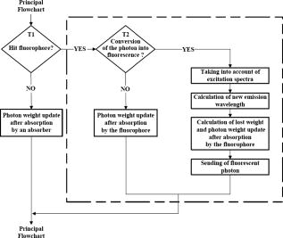

Considering an absorbing and diffusing medium containing $n_f$ fluorophores with absorption coefficients ${\mu }_{a{f}_i}\left(\lambda \right)$ and associated quantum yields ${\varphi }_i\left(\lambda \right)$ $(i∊[1,n_f])$ , the stepsize $\Delta s$ is calculated in the following way:

5.

$\Delta s=-\frac{\ln \xi }{{\mu }_t},$

$\text{with}{\mu }_t={\mu }_a+\sum _{i=1}^{n_f}{\mu }_{a{f}_i}+{\mu }_s,$

where $\xi ∊[0,1]$ is a random number generated from a uniform probability distribution.

At each absorption event, a first test $T_1$ is carried out to decide whether it is statistically due to a fluorescent compound (Fig. 2). The probabilities $p_{\mathit{abs}}$ that a photon is absorbed by a “pure” absorber and $p_{f_i}$ that a photon is absorbed by a fluorophore $f_i$ can respectively be defined as:

Eq. 6

$p_{\mathit{abs}}=\frac{{\mu }_a}{{\mu }_t}\text{and}{p}_{f_i}=\frac{{\mu }_{a{f}_i}}{{\mu }_t}.$

Therefore, a random number is calculated from a uniform distribution scaled with reference to the total probability of absorption $(p_{\mathit{abs}}+{\sum }_i{p}_{f_i})$ :

Eq. 7

${\xi }_{\mathrm{norm}}=\xi \times \left(\frac{{\mu }_a+{\sum }_i{\mu }_{a{f}_i}}{{\mu }_t}\right),$

and it is decided that the photon is absorbed either by a “pure” absorber if $0⩽{\xi }_{\mathrm{norm}}<p_{\mathit{abs}}$ , or by the fluorophore $f_i$ if:

Eq. 8

$p_{\mathit{abs}}+\sum _{i=0}^{n_f-1}{p}_{f_i}⩽{\xi }_{\mathrm{norm}}⩽p_{\mathit{abs}}+\sum _{j=i+1}^{n_f}{p}_{f_i}(p_{f_0}=0,n_f⩾2).$

In the first case (photon absorbed by a “pure” absorber), the photon’s weight becomes:

Eq. 9

${\omega }_a={\omega }_b(1-\frac{{\mu }_a}{{\mu }_a+{\sum }_i{\mu }_{a{f}_i}+{\mu }_s}),$

with ${\omega }_b,{\omega }_a$ being the photon weights before and after absor-ption.

In the second case (photon absorbed by a fluorophore $f_i$ ), a second test $T_2$ is performed to decide whether conversion into fluorescence happens, depending on the fluorophore quantum yield (Fig. 2). Again, the principle consists in generating a random number $\xi$ uniformly distributed between 0 and 1.

• • If this random number is higher than the quantum yield value $\varphi$ $(\varphi <\xi ⩽1)$ , then the incident photon is not converted into fluorescence. It continues its way until the next event, after having updated its energy level with reference to ${\mu }_{a{f}_i}$ as follows:

  Eq. 10

  ${\omega }_a={\omega }_b(1-\frac{{\mu }_{a{f}_i}}{{\mu }_a+{\sum }_i{\mu }_{a{f}_i}+{\mu }_s}).$

• • If $0⩽\xi ⩽\varphi$ , then the incident photon is fully absorbed and a new photon of fluorescence is generated at the same coordinates in the medium. The first propagation direction of the new emission photon is randomly sampled between 0 and $360\mathrm{deg}$ .

The emission wavelength of the new photon is also randomly sampled according to a probability distribution corres-ponding to the emission spectrum of the fluorophore, whatever the absorption wavelength. For example, if a fluorophore has an emission peak at a given wavelength, then the highest the probability emission of a fluorescence photon would be at this wavelength.

The values of the emission spectrum $S_{\mathit{em}}^{f_i}\left(\lambda \right)$ for each fluorophore $f_i$ being known, the following probability of emission of a fluorescence photon at a wavelength ${\lambda }_j$ is associated:

Eq. 11

$p\left[\text{photon}\left({\lambda }_j\right)\right]=v^{\prime }\left({\lambda }_j\right)=\frac{S_{\mathit{em}}\left({\lambda }_j\right)}{{\sum }_{j=1}^{n_p}{S}_{\mathit{em}}\left({\lambda }_j\right)},$

where $j∊[1,n_p]$ and $n_p$ accounts for the total number of points (wavelengths) used to discretize the emission spectrum.

A photon of fluorescence can cause another event of absorption fluorescence (the “cascade” effect). In addition, an incident photon absorbed at a wavelength ${\lambda }_{\mathit{abs}}$ cannot be converted into an emission photon with a wavelength lower than ${\lambda }_{\mathit{abs}}$ .

In the program based on the flowchart in Fig. 2, a specific file was created for each fluorophore in each layer, in which the values of the absorption and emission spectra, quantum yield, and absorption coefficient of fluorophores are stored. The simulation is made in the ascending way, i.e., from the lowest wavelength to the highest one, with $10\text{-}\mathrm{nm}$ sampling steps.

Finally, the function of cumulative distribution $C_{v^{\prime }}$ such as

$C_{v^{\prime }}\left({\lambda }_j\right)=\sum _{i=1}^j{v}^{\prime }\left({\lambda }_i\right),$

with $j∊[1,n_p]$ is used to choose the wavelength of emission in the following way:

Eq. 12

$\{\begin{array}{ll}\text{if}\xi ⩽C_{v^{\prime }}\left({\lambda }_1\right)& \Rightarrow \text{emission}\text{at}\text{wavelength}{\lambda }_1\\ \text{if}{C}_{v^{\prime }}\left({\lambda }_{j-1}\right)<\xi ⩽C_{v^{\prime }}\left({\lambda }_j\right)& \text{for}j⩾2,\\ & \Rightarrow \text{emission}\text{at}\text{wavelength}{\lambda }_j\end{array}\phantom{\}},$

with $\xi ∊[0,1]$ as a uniformly distributed random number.

2.3.

Test Phantoms

Phantoms were prepared with specific fluorophores, absor-ption, and scattering properties and dimensions, all of which are detailed hereafter. Liquid phantoms were made of absorber, scatterer, and one or two fluorophores, ethanol being used as thinner for the liquid phantoms since emission and absorption spectra of the fluorophores used here are given with ethanol as a thinner.³⁸ The relevance of the monofluorophore phantoms was to check the good correlation between measurements and simulation results. The relevance of multifluorophore phantoms was to check if the cascade effect was correctly taken into account. Then, multilayer solid phantoms were prepared in two and three layers with one or two fluorophores.

India ink (Super Black India ink, Lefranc/Bourgeois, France) was selected as the absorber. The absorption coefficient of pure India ink is available in Ref. 33, and the absor-ption coefficient of India ink diluted with water (Kabi-Fresenius) at 0.011% was measured using a spectrophotometer (Lambda EZ210, in DCPR Department of Physics Chemistry of the Reactions, Nancy, France).

Intralipids (Sigma Aldrich, Saint Louis, Missouri) were chosen as scatterer. They are often used as scatterers because they do not have a strong absorption band in the visible. They are made of intravenously administered nutrients consisting of an emulsion of phospholipid micelles and water, easily avai-lable and relatively inexpensive.^{36, 59, 60} The optical coefficients of intralipids are available in Ref. 36. Figure 3 represents the absorbance and the scattering coefficient as a function of wavelength for pure India ink and intralipids, respectively.

Fig. 3

(a) Pure India ink absorbance spectrum,³³ and (b) scattering coefficient of intralipids 10%.³⁶

Three fluorophores were selected for our experiments with reference to their distinct or partially overlapping emission spectra: eosin Y ( ${\mathrm{C}}_{20}{\mathrm{H}}_6{\mathrm{Br}}_4{\mathrm{Na}}_2{\mathrm{O}}_5$ , Sigma Aldrich), fluore-scein ( ${\mathrm{C}}_{20}{\mathrm{H}}_{12}{\mathrm{O}}_5$ , Fluka) and cryptocyanine ( ${\mathrm{C}}_{25}{\mathrm{H}}_{25}\mathrm{I}{\mathrm{N}}_2$ , Sigma Aldrich). Indeed, eosin Y dissolved in ethanol has a quantum yield of 0.67 at $490\mathrm{nm}$ , fluorescein a quantum yield of 0.79 at $425\mathrm{nm}$ , and cryptocyanine a quantum yield of 0.007 at $650\mathrm{nm}$ .³⁸ Moreover, fluorescein is referred to several articles for the creation and validation of equipment.^{61, 62}

Figure 4 represents the absorption spectrum of fluorescein, eosin, and cryptocyanine in ethanol for liquid phantoms,³⁸ and in water for solid phantoms, also measured in DCPR (Nancy).

Fig. 4

Fluorescein (bold solid line), eosin (solid line), and cryptocyanine (dotted line) absorption spectrum measured (a) in ethanol for liquid phantoms,³⁸ and (b) in water (spectrophotometer Lambda E270, DCPR, Nancy, France) for solid phantoms.

For all the phantoms, the fluorophores were systematically weighed to obtain a quantity of $10\mu \mathrm{mol}$ of product. All simulations were performed with 1,000,000 photons launched at 40 different wavelengths between 400 and $800\mathrm{nm}$ with $10\text{-}\mathrm{nm}$ steps (i.e., 40 million photons per spectrum), to ensure convergence of the results.

2.2.1.

Liquid phantoms

Four liquid phantoms were prepared: ${\mathrm{L}}_1$ ( $3.32\mathrm{mg}$ of fluorescein, $8\mathrm{mL}$ of ethanol), ${\mathrm{L}}_2$ ( $6.47\mathrm{mg}$ of eosin, $8\mathrm{mL}$ of ethanol), ${\mathrm{L}}_3$ ( $4.8\mathrm{mg}$ of cryptocyanine, $8\mathrm{mL}$ of ethanol), and ${\mathrm{L}}_4$ ( $3.32\mathrm{mg}$ of fluorescein, $4.8\mathrm{mg}$ of cryptocyanine in $16\mathrm{mL}$ of ethanol as thinner). All solution phantoms were poured into a black container comparable to one expanded polystyrene container, until reaching a height of $5\mathrm{mm}$ . The ${\mathrm{L}}_4$ phantom mixing two fluorophores was prepared to test the cascading effect itself (or secondary fluorescence emission due to another fluorescence photon).

2.2.2.

Solid mono- and multilayer phantoms

We used a solution of agarose (Agarose L, VWR Prolabo, France) at 5% ( $0.35\mathrm{mg}$ of agarose powder and $8\mathrm{mL}$ of distilled water) that has the property to become liquid at $82°\mathrm{C}$ and solid around $35°\mathrm{C}$ . Contribution of light scattering and fluorescence from agarose was checked to be negligible compared to the contributions of fluorophores at the wavelengths of excitation chosen for our experiments. Mono- and multilayer thicknesses were measured on sample sections with a Vernier micrometer (error: $\pm 0.02\mathrm{mm}$ ).

A first set of bilayered phantoms with one fluorophore ( ${\mathrm{MC}}_1$ , ${\mathrm{MC}}_2$ , and ${\mathrm{MC}}_3$ ) was prepared, having at the bottom (second layer, thickness $e_1=3\mathrm{mm}$ ) $3.32\mathrm{mg}$ of fluorescein and $0.35\mathrm{g}$ of agarose powder in $8\mathrm{mL}$ distilled water, and at the top (first layer, thickness $e_1=2.8\mathrm{mm}$ ) either $5\mathrm{mL}$ of India ink diluted at 0.011% $\left({\mathrm{MC}}_1\right)$ , or $5\mathrm{mL}$ of intralipids at 10% $\left({\mathrm{MC}}_2\right)$ , or a mixture of both $\left({\mathrm{MC}}_3\right)$ . For this set of phantoms, the first layer was kept in solution to prevent the optical properties from being modified by heating. A complementary single-layer phantom $\left({\mathrm{MC}}_4\right)$ was also made with $3.32\text{-}\mathrm{mg}$ fluorescein, $0.35\mathrm{g}$ of agarose powder, and $8\mathrm{mL}$ of distilled water (thickness $3\mathrm{mm}$ ) to compare the spectral res-ponses obtained for the previous bilayered phantoms with the ones of the second layer alone.

A second set of two- or three-layered phantoms was made with two different fluorophores. One bilayer phantom $\left({\mathrm{MC}}_5\right)$ was composed of $6.47\mathrm{mg}$ of eosin, $0.35\text{-}\mathrm{g}$ agarose, and $8\mathrm{mL}$ of water on the top layer (thickness $3\mathrm{mm}$ ), and of $3.32\mathrm{mg}$ of fluorescein, $0.35\mathrm{g}$ of agarose powder, and $8\mathrm{mL}$ of distilled water at the bottom layer (thickness $2.7\mathrm{mm}$ ). The trilayered phantom $\left({\mathrm{MC}}_6\right)$ was composed of a top layer of (thickness: $2.7\mathrm{mm}$ ) India ink diluted at 0.011%; a middle layer of (thickness $2\mathrm{mm}$ ) $6.47\mathrm{mg}$ of eosin, $0.35\mathrm{g}$ of aga-rose powder, and $8\mathrm{mL}$ of distilled water; and a bottom layer of (thickness $5.4\mathrm{mm}$ ) $3.32\mathrm{mg}$ of fluorescein, $0.35\mathrm{g}$ of agarose powder, and $8\mathrm{mL}$ of distilled water.

Table 1 recapitulates the characteristics and composition of the six types of multilayer phantoms tested.

Table 1

Characteristics of multilayer phantoms.

Phantom	MC1	MC2	MC3	MC4	MC5	MC6
First layer	$5\text{-}\mathrm{mL}$ India ink diluted at 0.011%	$5\text{-}\mathrm{mL}$ intralipids at 10%	$2.5\text{-}\mathrm{mL}$ solution 1		$6.47\text{-}\mathrm{mg}$ eosin
			$2.5\text{-}\mathrm{mL}$ solution 2		$0.35\text{-}\mathrm{g}$ agarose powder	solution 1
				—	$8\text{-}\mathrm{mL}$ distilled water
	(Solution 1)	(Solution 2)			(Solution 4)
		$e_1=2.8\mathrm{mm}$			$e_1=3\mathrm{mm}$	$e_1=2.7\mathrm{mm}$
Second layer		$3.32\text{-}\mathrm{mg}$ flurescein
		$0.35\text{-}\mathrm{g}$ agarose powder
		$8\text{-}\mathrm{mL}$ distilled water		—	Solution 3	Solution 4
		(Solution 3)
		$e_2=3\mathrm{mm}$			$e_2=2.7\mathrm{mm}$	$e_2=2\mathrm{mm}$
Third layer	—	—	—	Solution 3	—	Solution 3
				$e_3=3\mathrm{mm}$		$e_3=5.4\mathrm{mm}$

To quantify the difference between experimental and corresponding simulated spectra, we calculated, for all phantoms, the mean of normalized differences as follows:

Eq. 13

${\text{error}}_{\text{mean}}=\frac{1}{N}\sum _{i=1}^N\mid \frac{S_{\exp }\left({\lambda }_i\right)-S_{\mathrm{sim}}\left({\lambda }_i\right)}{S_{\exp }\left({\lambda }_i\right)}\mid ,$

with $N$ representing the number of curve points, $S_{\exp }\left(\lambda \right)$ the experimental reflectance spectrum, and $S_{\mathrm{sim}}\left(\lambda \right)$ the simulated reflectance spectrum.

3.

Results and Discussion

3.2.

Validation with Phantoms in Solution

All experiments were performed under monochromatic excitation with the laser diode source at $410\mathrm{nm}$ , except the phantom ${\mathrm{L}}_3$ performed with a a deuterium-tungsten halogen light source bandpass filtered at $650\pm 20\mathrm{nm}$ .

The correlation between simulated and measured emission spectra for each fluorophore was first verified using mono-fluorescence phantoms in solution (phantoms ${\mathrm{L}}_1$ , ${\mathrm{L}}_2$ , and ${\mathrm{L}}_3$ ). Experimental and simulation curves are shown in Fig. 5 . The spectra were normalized with reference to the maximum peak value of the spectra. Experimental and simulated spectra were normalized in the same way. A relatively good correlation was obtained, with error values of 2.2, 1.9, and 2.5% respectively for phantoms ${\mathrm{L}}_1$ , ${\mathrm{L}}_2$ , and ${\mathrm{L}}_3$ .

Fig. 5

Emission spectra measured (solid line) and simulated (squares) for single fluorophore phantoms ${\mathrm{L}}_1$ , ${\mathrm{L}}_2$ , and ${\mathrm{L}}_3$ made respectively of fluorescein/ethanol (bold solid line), eosin/ethanol (solid line), and cryptocyanine/ethanol (dotted line).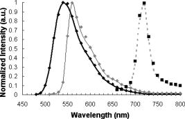

To test the proper operation of secondary fluorescence absorption (i.e., cascading fluorescence emission due to the absorption of another “already emitted” fluorescence photon), results in single excitation (phantoms ${\mathrm{L}}_1$ , ${\mathrm{L}}_3$ ) and multiple (or cascading) excitation (phantom ${\mathrm{L}}_4$ : fluorescein, cryptocyanine, ethanol) were compared (Fig. 6 ).

Fig. 6

Experimental (solid line) and simulated (squares) fluorescence spectra for a two-fluorophore phantom in solution ${\mathrm{L}}_4$ (fluorescein/cryptocyanine/ethanol).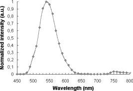

We observe that there is good correlation between experimental and simulated fluorescence spectra given in Fig. 6 with a mean error of 5.3%. For the phantom ${\mathrm{L}}_4$ and for the shortest distance between illumination and acquisition Fibers $\left(271\mu \mathrm{m}\right)$ , standard deviations for the experimental and simulated spectra (respectively ${\sigma }_{\exp }$ , ${\sigma }_{\mathrm{sim}}$ ) are:

$0.001\%<{\sigma }_{\exp }<5.9\%{\sigma }_{{\exp }_{\text{mean}}}\approx 0.8\%,$

$1.1\%<{\sigma }_{\mathrm{sim}}<5.3\%{\sigma }_{{\mathrm{sim}}_{\text{mean}}}\approx 1.9\%.$

For the longest distance between illumination and acquisition fibers $\left(1542\mu \mathrm{m}\right)$ , standard deviations are:

$0.05\%<{\sigma }_{\exp }<5.1\%{\sigma }_{{\exp }_{\text{mean}}}\approx 1.4\%,$

$1.5\%<{\sigma }_{\mathrm{sim}}<6.2\%{\sigma }_{{\mathrm{sim}}_{\text{mean}}}\approx 2.1\%.$

The results obtained were verified and were of the same order of magnitude for all other distances.

The emission intensity spectra of fluorescein between 480 and $650\mathrm{nm}$ (peak at $540\mathrm{nm}$ ) and of cryptocyanine at wavelengths above $700\mathrm{nm}$ (emission peak at $730\mathrm{nm}$ ) can be clearly noticed, and their proportional contributions are well reproduced by the simulation algorithm including cascading fluorescence. With reference to the absorption spectrum of cryptocyanine, we can even check in Fig. 6 that the amplitude of the fluorescein emission spectrum is clearly decreased in the $580\text{to}700\text{-}\mathrm{nm}$ wavelength band compared to the one of phantom ${\mathrm{L}}_1$ in Fig. 5, indicating that absorption by cryptocyanine occurs and therefore that the cascade effect does exist.

3.3.

Validation with Multilayered Phantoms

Experimental and simulated fluorescence spectra for multilayered phantoms ${\mathrm{MC}}_1$ (India ink/fluorescein), ${\mathrm{MC}}_2$ (intralipids/fluorescein), ${\mathrm{MC}}_3$ (India ink/intralipids/fluorescein) and ${\mathrm{MC}}_4$ (fluorescein) are given in Fig. 7 . The latter also highlights the way in which the fluorescence spectra are modified by the presence of absorbing and diffusing layers. Experimental spectra were normalized with reference to the maximum peak value of the experimental value of phantom ${\mathrm{MC}}_4$ , and simulated spectra with reference to the maximum peak value of the simulated value of phantom ${\mathrm{MC}}_4$ .

Fig. 7

From top to bottom: experimental (solid line) and simulated (squares) fluorescence spectra for phantoms ${\mathrm{MC}}_4$ (fluorescein), ${\mathrm{MC}}_1$ (India ink/fluorescein), ${\mathrm{MC}}_3$ (India ink/intralipids/fluorescein), and ${\mathrm{MC}}_2$ (intralipids/fluorescein).

Looking comparatively at the spectra of ${\mathrm{MC}}_4$ and ${\mathrm{MC}}_1$ phantoms, it can be noticed that the addition of a purely absorbing top layer (India ink) leads to a global amplitude attenuation, while the overall shape of the spectrum remains similar. By comparing ${\mathrm{MC}}_4$ and ${\mathrm{MC}}_2$ spectra, we may observe that the presence of a diffusing top layer (intralipids) causes strong attenuation of the collected signal and also a change in the shape of the curve. In the case of phantom ${\mathrm{MC}}_3$ , the absorbing and diffusing top layer leads to attenuation and shape modification of the reflected spectra.

For these four different configurations, the results obtained experimentally and by simulation agree well. The lowest mean percent error obtained between experimental and simulated spectra is 2.5% for phantom ${\mathrm{MC}}_4$ (fluorescein), 6.0% for ${\mathrm{MC}}_2$ (intralipids, fluorescein), 7.1% for ${\mathrm{MC}}_1$ (India ink, fluorescein), and the maximum mean percent error is 9.4% for ${\mathrm{MC}}_3$ (India ink, intralipids, fluorescein). It can be noticed that the mean percent error is slightly higher for the solid phantom ${\mathrm{MC}}_4$ (2.5%) than for the phantom ${\mathrm{L}}_1$ in solution (2.2%).

Figure 8 represents the measured and simulated fluore-scence spectra for the bilayers phantom ${\mathrm{MC}}_5$ with two fluorophores (eosin on the top layer and fluorescein at the bottom layer) and for the trilayer phantom ${\mathrm{MC}}_6$ with the same two fluorophore layers and an upper absorbing layer (India ink/eosin/fluorescein). A few explanations can be given as to the shape changes of spectra in Fig. 8. As presented in Fig. 3a, India ink absorbs twice as much at $400\mathrm{nm}$ as at $800\mathrm{nm}$ , therefore altering the spectrum unequally over the wavelength band. Thus, the eosin fluorescence appears proportionally with more intensity than the fluorescein fluorescence. Consequently, the modification of the shape in Fig. 8 is due to the absorption spectra of India ink and to the fact that this was added in a supplementary top layer. The mean percent error calculated between experimental and simulated spectra is 9.3% for the bilayer phantom ${\mathrm{MC}}_5$ with two fluorophores (eosin, fluorescein) and 10.6% for the trilayer phantom ${\mathrm{MC}}_6$ (India ink, eosin, fluorescein). It should be noted that the mean percent error increases with the addition of an absorbing layer, and with the number of layers (increased thickness). This trend is confirmed for the 12 other distances between illumination and acquisition fibers $\left(340\text{to}1542\mu \mathrm{m}\right)$ . For the $528\text{-}\mu \mathrm{m}$ interfiber distance, the average error varies from 3.1% for ${\mathrm{MC}}_4$ to 10.9% for ${\mathrm{MC}}_6$ . We can observe that the mean percent error values increase with the interfiber distances and with the medium complexity, i.e., the number of collected photons. Given the number of absorbing, fluore-scing, or diffusing layers, the increases in average error are probably due to the relative increase of statistical noise inherent to Monte Carlo simulation, because we used the same number of photons for all simulations (40 million photons per spectrum) whatever the phantom complexity.

Fig. 8

Measured (solid line) and simulated (squares) fluorescence spectra for a bilayer phantom ${\mathrm{MC}}_5$ (bold solid line) with two fluorophores (eosin in top layer, and fluorescein in bottom layer), and for a trilayer phantom ${\mathrm{MC}}_6$ (dotted line) with the same two fluorophores but with an upper absorbing layer added (India ink/eosin/fluorescein).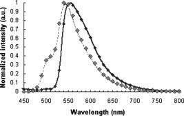

Execution times vary with the composition of the phantoms, and more particularly with the optical parameters used in the simulation. Using a pentium 4, $2.4\text{-}\mathrm{GHz}$ and 512-Mo RAM computer, execution times (20 million photons per spectra) range from $6\min$ for ${\mathrm{MC}}_4$ (fluorescein, agarose) to $34\min$ for three-layered phantom ${\mathrm{MC}}_6$ with two fluorophores (India ink, eosin, fluorescein). Simulation time is doubled between the monolayer monofluorophore phantom ${\mathrm{MC}}_4$ and bilayer bifluorophore ${\mathrm{MC}}_5$ $\left(15\min \right)$ .

4.

Conclusion

Anatomical, physiological, and biochemical changes result in modifications of the absorption and light scattering in pathological tissues compared to healthy ones. These local changes of the optical properties affect the characteristics of reflectance diffuse spectra. The measurement of endogenous and exogenous fluorescence from tissue has become a very useful research and clinical diagnostic tool. Many authors have shown that fluorescence can indicate the presence of mali-gnant tissue, but one of the major limitations is that the fluorescence signal is mixed with absorption and scattering, which is intrinsic to the tissue components. As a consequence, Monte Carlo methods are widely used to model the fluore-scence emitted by the tissues. Part of the difficulty lies in the coupled simulation of absorption, diffusion, and multiple fluorescence in a multilayer medium, over a broad spectral band.

In this work, a Monte Carlo algorithm is developed for simulating the spectral absorption, diffusion, and multiple fluorescence in a multilayer medium, over a broad spectral band. As a primary validation, the correct operation of our program, including our fluorescence algorithm, is first verified in relation to other Monte Carlo simulation results referenced in literature for absorption and diffuse reflectance without fluorescence (same parametrization). The main experimental validation consists in comparing the fluorescence spectra measured on phantoms of various complexities to Monte Carlo simulated spectra of their corresponding models (mono- and multilayered). Four phantoms in solution with three different fluorophores and six mono- and multilayered solid phantoms with one or two fluorophores are used. The good correlation between simulated and experimentally measured results is quantified on the basis of mean error calculations. For phantoms in solution, the mean percent errors vary from 1.9% (one fluorophore) to 5.3% (two fluorophores). For multilayered phantoms, these errors range from 6.0% (two layers), to 9.4% for the trilayer phantom. The error values vary according to the complexity of the phantom, i.e., the model (for a fixed number of photons launched). Finally, the proper operation of “secondary fluorescence” (fluorescence emission due to the absorption of another already emitted fluorescent photon) is demonstrated.

This model proves appropriate for applications to biological tissues, in which the contribution of absorbers, scatterers, and fluorophores vary. More specifically, this work will be used for in-vivo tissue diagnosis such as precancer and cancer detection, where the identification of proper values of the optical parameters for these tissues takes into account the associated phenomenon of multiple fluorescence.