Wavelet minimum description length detrending for near-infrared spectroscopy

Kwang-Eun Jang; Sungho Tak; Jinwook Jung; Jaeduck Jang; Yong Jeong; Yong Chul Ye

doi:10.1117/1.3127204

1 May 2009 Wavelet minimum description length detrending for near-infrared spectroscopy

Kwang-Eun Jang, Sungho Tak, Jinwook Jung, Jaeduck Jang, Yong Jeong, Yong Chul Ye

Author Affiliations +

Journal of Biomedical Optics, Vol. 14, Issue 3, 034004 (May 2009). https://doi.org/10.1117/1.3127204

Abstract

Near-infrared spectroscopy (NIRS) can be employed to investigate brain activities associated with regional changes of the oxy- and deoxyhemoglobin concentration by measuring the absorption of near-infrared light through the intact skull. NIRS is regarded as a promising neuroimaging modality thanks to its excellent temporal resolution and flexibility for routine monitoring. Recently, the general linear model (GLM), which is a standard method for functional MRI (fMRI) analysis, has been employed for quantitative analysis of NIRS data. However, the GLM often fails in NIRS when there exists an unknown global trend due to breathing, cardiac, vasomotion, or other experimental errors. We propose a wavelet minimum description length (Wavelet-MDL) detrending algorithm to overcome this problem. Specifically, the wavelet transform is applied to decompose NIRS measurements into global trends, hemodynamic signals, and uncorrelated noise components at distinct scales. The minimum description length (MDL) principle plays an important role in preventing over- or underfitting and facilitates optimal model order selection for the global trend estimate. Experimental results demonstrate that the new detrending algorithm outperforms the conventional approaches.

1. Introduction

Near-infrared (NIR) light, with a wavelength between $650 nm$ and $950 nm$ , is capable of penetrating deeply through biological tissues. This is because NIR light is weakly absorbed by biological chromophores such as hemoglobin, myoglobin, and cytochrome c oxidase.¹ The relatively deep penetration depth of NIR light in the human brain makes it possible to measure brain activities associated with regional changes of oxy- and deoxy hemoglobin concentrations.² This spectroscopic technique using NIR light for monitoring brain activities is known as functional near-infrared spectroscopy (NIRS).³

NIRS is regarded as a promising neuroimaging modality owing to a number of advantages over other neuroimaging modalities such as positron emission tomography (PET) and functional magnetic resonance imaging (fMRI).³ For example, there is no theoretical limitation on temporal resolution (while of course there are practical limits arising from, for example, the speed of the analog-to-digital converter). The temporal resolution of NIRS, therefore, is sufficient to investigate hemodynamic responses due to brain activations as well as other fast varying physiological conditions. Furthermore, NIRS does not require that the subject lie on his/her back in a confined environment during experiments, thereby making it possible to investigate subjects that would normally be difficult to examine using fMRI or PET, including infants, children, and patients with psychological issues. Moreover, NIRS is highly flexible, portable, and relatively low cost.

However, there remain several theoretical and practical difficulties for quantitative analysis of NIRS data. For example, the differential path length factor (DPF)⁴ depends on various parameters such as the age of the subject,⁵ wavelength of the imaging system,⁶ and position within a brain.⁷ Time-resolved or frequency domain NIRS equipment may be used to estimate the mean optical path length; however, continuous wave (CW) systems are more commonly used due to several practical concerns such as cost of implementation.⁷ Other subject-dependent parameters such as depth of the skull and optical properties of hair may influence measurement of optical parameters.

Recently, many researchers have been developing statistical analysis toolboxes for NIRS based on the generalized linear model (GLM).^{8, 9, 10, 11} The GLM is a statistical linear model that explains data as a linear combination of explanatory variables plus an error term. Since the GLM analysis relies on the temporal variational pattern of signals, it is more robust to differential path length factor (DPF) variation, optical scattering, or poor contact. Furthermore, statistical parameter mapping (SPM) using the GLM is a standard method for analyzing fMRI data,¹² and thus integration of NIRS and fMRI within the same SPM framework may offer the advantage of modeling both types of data in the same mathematical framework to make inferences. Based on these observations, we have developed a new public domain statistical toolbox called NIRS-SPM.¹¹ By incorporating the GLM with the $p$ -value calculation using Sun’s tube formula,^{13, 14} NIRS-SPM not only enables calculation of activation maps of oxy-, deoxy, and total hemoglobin but also allows for super resolution localization, which is not possible using conventional analysis tools.¹¹

Note that the GLM often fails when there exist global drifts in the NIRS measurements due to various reasons, such as subject movement, blood pressure variation, and instrumental instability. This global trend causes a low-frequency bias in NIRS measurements. Moreover, the amplitude of the global drift is often comparable to that of the signal from brain activation, which degrades the signal-to-noise ratio. In order to eliminate the global trend and thus improve the signal-to-noise ratio, high-pass filtering is often used in practice.¹⁵ However, the signals from brain activations are often degraded by a simple filtering, since the frequency response of the hemodynamic response can also be affected during high-pass filtering.

In order to overcome this problem, this paper investigates a wavelet-based detrending algorithm for fMRI¹⁶ and adapts it for NIRS applications. Specifically, the wavelet transform was applied to decompose NIRS measurements into global trends, hemodynamic signals, and noise components at distinct scales. However, unlike fMRI data, the NIRS time series is considerably long due to the fast sampling frequency. Hence, we observed that direct application of the model order selection rule in Ref. 16 leads to erroneous results in NIRS. To remedy this problem, the minimum description length (MDL) principle with universal prior of integers¹⁷ is found to be suitable for the NIRS time series, as it avoids over- and underfitting of the global trend estimate, thanks to the asymptotic optimality of MDL. Experimental results confirm that the new detrending algorithm outperforms the conventional approaches. We have therefore incorporated the proposed Wavelet-MDL detrending algorithms within our NIRS-SPM framework, which will soon be publicly available at the website of the authors (http://bisp.kaist.ac.kr/NIRS-SPM). We observed that the Wavelet-MDL detrending method within NIRS-SPM provides more specific localizations of the neuronal activation than the standard high-pass filtering approach based on the discrete cosine transform (DCT).

2. NIRS Measurement Model

The modified Beer-Lambert law (MBLL), which describes optical attenuation in a highly scattering medium such as biological tissue,⁴ provides a relation between raw optical density (OD) data and changes of chromophore concentrations. According to the MBLL, the change in $OD (λ, r, t)$ for the wavelength $λ$ at the cerebral cortex position $r ∊ R^{3}$ at time $t$ due to the $N_{c}$ number of chromophore concentration changes ${[Δ c^{(i)} (r, t)]}_{i = 1}^{N_{c}}$ is described as

Eq. 1

Δ OD (λ, r, t) = - \ln (\frac{I_{F}}{I_{o}}) = \sum_{i = 1}^{N_{c}} a_{i} (λ) Δ c^{(i)} (r, t) d (r) l (r),

where

I_{F}

denotes the final measured optical intensity,

I_{o}

denotes the initial measured optical intensity,

a_{i} (λ)

is the extinction coefficient of the

i

’th chromophore at wavelength

λ

,

d (r)

is the DPF, and

l (r)

is the distance between the source and detector at position

r

, respectively. Assuming that oxy- and deoxyhemoglobin are the major two choromophores, the noisy measured optical density is then described by the following matrix formulation:

Eq. 2

[\begin{matrix} Δ OD (r, t; λ_{1}) \\ Δ OD (r, t; λ_{2}) \end{matrix}] = d (r) l (r) [\begin{matrix} a_{1} (λ_{1}) & a_{2} (λ_{1}) \\ a_{1} (λ_{2}) & a_{2} (λ_{2}) \end{matrix}] [\begin{matrix} Δ c_{Hb O} (r, t) \\ Δ c_{Hb R} (r, t) \end{matrix}] + [\begin{matrix} w (r, t; λ_{1}) \\ w (r, t; λ_{2}) \end{matrix}],

where

Δ c_{Hb O} (r, t)

and

Δ c_{Hb R} (r, t)

denote the time series of the chromophore changes for the oxy- and deoxyhemoglobin, and

w (r, t; λ_{i})

is the additive noise for the wavelength

λ_{i}

, respectively. Here, we assume that

d (r)

is the same at both wavelengths and the equality assumption does not affect the validity or applicability of what follows. Then, by multiplying the inverse matrix of the extinction coefficients with Eq. 2, we can derive the expression of the noisy oxy- and deoxyhemoglobin signals:

Eq. 3

[\begin{matrix} y_{Hb O} (r, t) \\ y_{Hb R} (r, t) \end{matrix}] = d (r) l (r) [\begin{matrix} Δ c_{Hb O} (r, t) \\ Δ c_{Hb R} (r, t) \end{matrix}] + [\begin{matrix} ϵ_{Hb O} (r, t) \\ ϵ_{Hb R} (r, t) \end{matrix}],

where

ϵ_{Hb O} (r, t)

and

ϵ_{Hb R} (r, t)

is the additive zero mean Gaussian noise for the oxy- and deoxy- channels, respectively. Although the DPF parameter

d (r)

can be measured using time-domain or frequency-domain systems by calculating the temporal point spread function,⁷ this information is not obtainable in commonly available CW systems. Furthermore, NIRS data acquisition is considerably affected by a variety of measurement conditions, such as the color of hair and the scalp depth, which introduces position- and subject-dependent scattering effects. For these reasons, analyzing NIRS data using the magnitude of chromophore concentration changes is often problematic.

3. General Linear Model for NIRS

In the fMRI domain, the validity of the GLM has been extensively tested, and the GLM has been established as a standard analyzing method. Statistical parametric mapping (SPM)¹⁸ and analysis of functional neuro images (AFNI)¹⁹ are widely used programs based on the GLM. Analysis based on the GLM consists of three steps: model specification, parameter estimation, and statistical inference.¹⁵ In this section, we review the GLM approach for NIRS applications.¹¹

The GLM describes a measurement $y_{Hb X} (r, t)$ (i.e., $y_{Hb O}$ or $y_{Hb R}$ ) in terms of a linear combination of $L$ explanatory variables plus an error term:

Eq. 4

y_{Hb X} (r, t) = x_{1} (t) β_{1} + \dots + x_{L} (t) β_{L} + ϵ_{Hb X} (r, t) .

Here,

β_{i}

denotes an unknown strength of response, and

x_{i} (t)

is an explanatory variable originating from a model of hemodynamic responses. Now, let

y

and

ϵ

denote the vector of the time series of the hemodynamic signal and noise at the location

r

, respectively:

Eq. 5

y = {[y_{Hb X} (r, t_{1}) y_{Hb X} (r, t_{2}) \dots y_{Hb X} (r, t_{N})]}^{T},

Eq. 6

ϵ = {[ϵ_{Hb X} (r, t_{1}) ϵ_{Hb X} (r, t_{2}) \dots ϵ_{Hb X} (r, t_{N})]}^{T} .

The corresponding GLM model in a matrix form is then given by:

Eq. 7

y = X β + ϵ,

where

y

is an

N

-dimensional column vector whose elements are the sampled NIRS data at

N

time points,

ϵ

denotes an error vector, and

β

is an

L

-dimensional column vector that represents unknown strengths of the response. Usually, the

N \times L

matrix

X

is called a design matrix and serves as a predictor for the measured signal.¹⁵

For fMRI signals, Boynton showed that the BOLD signal can be approximated as a convolution model between a stimulus function and a hemodynamic response function (HRF).²⁰ Based on a similar argument, several statistical analysis toolboxes using the GLM are currently available for NIRS.^{8, 9, 10, 11} The stick function or the boxcar function is typically used for the stimulus function. For the HRF, there are a number of possible models. In this paper, we follow fMRI approaches and employ the so-called canonical HRF, which is composed of two gamma functions.¹⁵ Additionally, the derivatives of the HRF with respect to delay and dispersion can be used to mitigate the problem that the precise shape of the HRF varies across the brain.²¹ An adaptive estimation of HRF using multiple gamma functions can also be used in NIRS to account for oxygen species–dependent hemodynamics variation.¹¹

After the model specification, the least-squares parameter estimator is derived using the ordinary least squares. If the design matrix $X$ is of full rank, the least-squares estimate is:

Eq. 8

\hat{β} = {(X^{T} X)}^{-} X^{T} y,

where

X^{-}

denotes the pseudo-inverse of

X

. With the obtained least-squares estimates, one can construct statistics for the statistical inference. In most cases, we consider a linear combination of the parameter estimates:

Eq. 9

c_{1} {\hat{β}}_{1} + \dots + c_{L} {\hat{β}}_{L} = c^{T} \hat{β},

where the vector

c

is called a contrast vector.¹⁵ Similar to the fMRI-SPM analysis,¹⁵ the error

ϵ

in Eq. 7 is assumed to be normally distributed with a temporal covariance matrix

Σ

; hence, we have

Eq. 10

c^{T} \hat{β} \sim N [c^{T} β, c^{T} {(X^{T} X)}^{-} X^{T} Σ X {(X^{T} X)}^{-} c] .

Thus,

t

-statistics for the null hypothesis that asserts no activation is given by

Eq. 11

t = \frac{c^{T} \hat{β}}{{[c^{T} {(X^{T} X)}^{-} X^{T} Σ X {(X^{T} X)}^{-} c]}^{1 ∕ 2}},

where

t

denotes a random variable with a Student’s

t

-distribution with degree of freedom

df

given as follows:¹⁵

Eq. 12

df = \frac{tr {[R Σ]}^{2}}{tr [R Σ R Σ]}, R = I_{N \times N} - X {(X^{T} X)}^{-} X^{T},

where

I_{N \times N}

denotes the

N \times N

identity matrix.

The estimate of the temporal correlation matrix $Σ$ hence affects the overall $t$ -value and corresponding inferences. For a detailed discussion on the estimation of $Σ$ , readers can refer to our previous work on this issue.¹¹ If the calculated $t$ -value is larger than a certain threshold value, then the inference steps abandon the null hypothesis and we declare the area to be activated. The threshold value is calculated by fixing a $p$ -value in the range of 0.001 to 0.05. A smaller $p$ -value provides a higher threshold value. The nonlinear relationship between the $p$ -value and threshold can be explicitly represented using the tube formula, as described in our companion paper.¹¹

4. Wavelet-MDL Detrending

In this section, we develop a novel detrending algorithm that is designed to address the global-drift issues described in the Introduction. Our point of departure is an algorithm developed for detrending the fMRI time series.¹⁶

4.1.

Notation

We first introduce the notation associated with a discrete wavelet transform by following the standard conventions.²² Let $ψ (t)$ denote a wavelet associated with the multiresolution analysis.²² Let $Φ (t)$ , $h$ , and $g$ be the scaling function, the low-pass filter, and the high-pass filter associated with this wavelet transform, respectively. With a slight abuse of notation, let $θ = {θ [n]}, n = 0, \dots, N - 1$ be a discrete version of a continuous signal $θ (t)$ . For simplicity, we assume $N = 2^{J}$ , where $J$ is the maximum level of wavelet decomposition. The wavelet coefficients composed of approximation coefficients ${a θ_{j} [k]}_{j, k}$ and detail coefficients ${d θ_{j} [k]}_{j, k}$ are defined by the following recursions:²²

a θ_{0} [k] = θ [k], k = 0, \dots, N - 1,

a θ_{j + 1} [k] = \sum_{n} h [n - 2 k] a θ_{j} [n], k = 0, \dots, 2^{- j - 1} N - 1,

d θ_{j + 1} [k] = \sum_{n} g [n - 2 k] a θ_{j} [n], k = 0, \dots, 2^{- j - 1} N - 1,

where

j = 0, \dots, J - 1

. We introduce a matrix

W

to represent the discrete wavelet transform:

Eq. 13

W θ = {a θ_{J} [0], d_{J}, d_{J - 1}, \dots, d_{1}}^{T},

where each submatrix is given by

d_{J} = {d θ_{J} [0]} ∊ R^{1 \times 1},

d_{J - 1} = {d θ_{J - 1} [0], d θ_{J - 1} [1]}^{T} ∊ R^{2 \times 1},

d_{j} = {d θ_{j} [0], \dots, d θ_{j} [2^{- j} N - 1]}^{T} ∊ R^{2^{- j} N \times 1},

d_{1} = {d θ_{1} [0], \dots, d θ_{1} [2^{- 1} N - 1]}^{T} ∊ R^{2^{- 1} N \times 1} .

4.2.

Modified GLM with Baseline Drift

In the wavelet detrending algorithm for fMRI,¹⁶ the baseline drift is included as part of the GLM:

Eq. 14

y = X β + ϵ + θ,

where

y

indicates the measured BOLD signal,

X

and

ϵ

denote the predictor and the additive noise with the temporal covariance matrix

Σ

, and

θ

is the additional global drift, respectively. A similar argument may be applied to the NIRS case. We introduce trend terms in Eq. 2 as follows:

Eq. 15

[\begin{matrix} Δ OD (r, t; λ_{1}) \\ Δ OD (r, t; λ_{2}) \end{matrix}] = d (r) l (r) [\begin{matrix} a_{1} (λ_{1}) & a_{2} (λ_{1}) \\ a_{1} (λ_{2}) & a_{2} (λ_{2}) \end{matrix}] [\begin{matrix} Δ c_{Hb O} (r, t) \\ Δ c_{Hb R} (r, t) \end{matrix}] + [\begin{matrix} w (r, t; λ_{1}) \\ w (r, t; λ_{2}) \end{matrix}] + [\begin{matrix} \tilde{θ} (r, t; λ_{1}) \\ \tilde{θ} (r, t; λ_{2}) \end{matrix}],

where

\tilde{θ} (r, t; λ_{i})

denotes the global trend for wavelength

λ_{i}

at the location

r

. If we multiply the inverse matrix of the extinction coefficients, the equation of the noisy oxy- and deoxyhemoglobin is given as

Eq. 16

[\begin{matrix} y_{Hb O} (r, t) \\ y_{Hb R} (r, t) \end{matrix}] = d (r) l (r) [\begin{matrix} Δ c_{Hb O} (r, t) \\ Δ c_{Hb R} (r, t) \end{matrix}] + [\begin{matrix} ϵ_{Hb O} (r, t) \\ ϵ_{Hb R} (r, t) \end{matrix}] + [\begin{matrix} θ_{Hb O} (r, t) \\ θ_{Hb R} (r, t) \end{matrix}],

where

θ_{Hb O} (r, t) = 1 ∕ C [a_{2} (λ_{2}) \tilde{θ} (r, t; λ_{1}) - a_{2} (λ_{1}) \tilde{θ} (r, t; λ_{2})]

,

θ_{Hb R} (r, t) = 1 ∕ C [- a_{1} (λ_{2}) \tilde{θ} (r, t; λ_{1}) + a_{1} (λ_{1}) \tilde{θ} (r, t; λ_{2})]

, and

C = [a_{1} (λ_{1}) a_{2} (λ_{2}) - a_{2} (λ_{1}) a_{1} (λ_{2})]

. Let

y_{Hb X}

,

ϵ_{Hb X}

, and

θ_{Hb X}

denote vectors of the hemodynamic signal, additive noise, and global trend signal, respectively. If we introduce the GLM for each chromophore, we can derive the modified GLM for NIRS as follows:

Eq. 17

y_{Hb X} = X_{Hb X} β_{Hb X} + ϵ_{Hb X} + θ_{Hb X} .

For simplicity, we remove the subscript

Hb X

from Eq. 17 and use the general form given by Eq. 14.

The global trend signal varies smoothly in most cases. Based on this observation, conventional detrending algorithms use filtering to remove the low-frequency trend signal. The problem of this approach, however, is that the hemodynamic signal often has a low-frequency varying component that can be erroneously removed during the filtering. In order to deal with this artifact, in our wavelet detrending, the unknown trend is modeled as a signal restricted in a subspace spanned by coarse scale wavelets.¹⁶ More specifically, the trend is modeled as:¹⁶

Eq. 18

θ (t) = a θ_{J} [0] Φ (2^{- J} t) + \sum_{j = J_{0}}^{J} \sum_{k = 0}^{2^{- j} N - 1} d θ_{j} [k] ψ (2^{- j} t - k),

where

Φ

,

ψ

,

a θ_{J}

,

d θ_{j}

,

J

, and

N

are defined as earlier, and

J_{0}

denotes the finest scale that determines the smoothness of the trend. Note that the detail coefficients

d θ_{j} [k]

are all zero for fine scales, i.e.,

1 ⩽ j ⩽ J_{0} - 1

.

Using the discrete wavelet transform (DWT) matrix $W$ defined in Eq. 13, we can represent the wavelet transform of a global trend signal as follows:

Eq. 19

W θ = {[a θ_{J} [0], d_{J}, \dots, d_{J_{0}}, 0, \dots, 0]}^{T} .

The maximum likelihood estimates for the trend

θ

and the unknown signal strength

β

in Eq. 14 are then given by:¹⁶

Eq. 20

\hat{ξ} = {[A^{T} Σ^{- 1} A]}^{- 1} A^{T} Σ^{- 1} W y,

where

ξ = {a θ_{J} [0], d θ_{J} [0], \dots, d θ_{J_{0}} [2^{- J_{0}} N - 1], β}^{T}

, and

A = [\begin{matrix} 1 & 0 & a x_{J}^{(1)} [0] & \dots & a x_{J}^{(L)} [0] \\ 1 & 0 & x_{J}^{(1)} & x_{J}^{(L)} \\ \dots & ⋮ & ⋮ & \dots & ⋮ \\ 1 & 0 & ⋮ & ⋮ \\ 1 & x_{J_{0}}^{(1)} & \dots & x_{J_{0}}^{(L)} \\ 0 & x_{J_{0} - 1}^{(1)} & x_{J_{0} - 1}^{(L)} \\ ⋮ & ⋮ & \dots & ⋮ \\ 0 & x_{1}^{(1)} & \dots & x_{1}^{(L)} \end{matrix}] = [\begin{matrix} I_{n_{0} \times n_{0}} \\ W X \\ 0_{(N - n_{0}) \times n_{0}} \end{matrix}],

where

n_{0} = 2^{- J_{0} + 1} N

denotes the number of nonzero coefficients that describe the trend,

I_{n_{0} \times n_{0}}

denotes a

n_{0} \times n_{0}

identity matrix,

0_{(N - n_{0}) \times n_{0}}

denotes a

(N - n_{0}) \times n_{0}

matrix whose elements are zero,

A

is a

N \times (n_{0} + L)

matrix,

Σ

denotes the

N \times N

noise covariance matrix,

W

is the DWT matrix, and

x_{i}^{(k)}

is the

i

’th wavelet coefficient of the

k

’th column of design matrix, respectively.

Note that $Σ$ in Eq. 20 is the covariance matrix of noise in wavelet domain. Even if the original time series is highly correlated, the array of wavelet coefficients exhibits much less correlation.²³ This decorrelating (or whitening) feature of the wavelet transform has been studied in Refs. 23, 24, 25. Especially for the fractional Brownian motion (fBM) process,²⁶ which is a popular model for $1 ∕ f$ -type noise, the decay rate of the correlation of wavelet coefficients in $j$ ’th scale is derived as:²⁴

Eq. 21

E {d θ_{j} [m], d θ_{j} [n]} = O ({∣ 2^{- j} (m - n) ∣}^{2 (H - p)}),

where

E {\cdot}

is an expectation operator,

H ∊ (0.5,1)

is a constant that defines the degree of correlation, and

p

denotes the number of vanishing moments of a wavelet transform. Therefore, for a wavelet transform that has a large enough

p

, we may assume that the noise in wavelet coefficients has the uncorrelated Gaussian distribution whose covariance matrix is given as:

Eq. 22

Σ = diag {σ_{J}^{2}, σ_{J}^{2}, \dots, σ_{1}^{2}},

where

σ_{j}^{2}

is the variance in the

j

’th decomposition level. To estimate

σ_{j}^{2}

, we use the median absolute deviation of wavelet coefficients:^{23, 27}

Eq. 23

{\hat{σ}}_{j}^{2} = Median {d θ_{j} [0], \dots, d θ_{j} [2^{- j} N - 1]} ∕ 0.6745,

where the number 0.6745 is the calibration factor for Gaussian distribution.^{23, 27}

In the wavelet detrending method for a fMRI time series,¹⁶ the complexity of the unknown global bias is solely determined by $J_{0}$ . In other words, there is an implicit assumption that all coefficients at the same scale are all zero or all nonzero simultaneously. However, in the case of NIRS, the number of data points $N$ is much larger than that of the fMRI time series, and thus this simple scheme may cause over- or underfitting. Therefore, for a fine-tuned estimate of model order, the wavelet coefficients at the same scale are sorted in order of descending magnitude and are included one by one until a suitable complexity is found by the model order selection criterion. Note that this procedure is similar to MDL thresholding in signal restoration.^{28, 29}

The wavelet detrending method has several advantages over the conventional filtering approach. Note that the conventional filtering cannot prevent the removal of the hemodynamic signal, since it decides the cutoff frequency using only the paradigm repetition frequency, and the nonnegligible amount of the hemodynamic signals can often be filtered out. This is especially true for the event-related paradigm³⁰ since it does not have a well-defined cutoff frequency. Compared with the conventional method, the wavelet-based detrending algorithm includes the design matrix $X$ in the least-squares estimation process described in Eq. 20. Hence, the canonical hemodynamics time series is fully utilized in the estimation process, and the algorithm is more robust. Furthermore, the wavelet-based approach is more effective in removing relatively fast varying trends thanks to the optimality of wavelet transform in describing the transient changes of fast varying signals.²²

4.3.

Minimum Description Length Principle for Model Order Selection

In Eq. 20, we have shown a simple one-step method for simultaneous estimation of the global trend $θ$ and the signal strength $β$ for a given hyperparameter $J_{0}$ in terms of maximum likelihood estimation. The remaining issue is the determination of the hyperparameter $J_{0}$ . Even though $J_{0}$ is a single integer valued parameter, it affects the whole behavior of the estimated trend signal, since $J_{0}$ determines the number of wavelet coefficients $n_{0}$ that describe the trend. More specifically, if $n_{0}$ is an inappropriately large number, the hemodynamic response is distorted due to the overfitted trend estimate, whereas a smaller $n_{0}$ value may not capture the unknown trend properly. Therefore, the accuracy of the order estimate $J_{0}$ (or $n_{0}$ ) ultimately determines the quality of the trend estimation.

The problem of estimating the order $J_{0}$ (or $n_{0}$ ) is formally called the model order selection problem.^{17, 31, 32} A good model order selection criterion should satisfy two conflicting goals simultaneously: goodness of fit and concision of the model. Balancing these two goals is crucial in preventing the over- or underfitting. Akaike information criterion (AIC),³³ Schwartz information criterion (SIC),³² and minimum description length (MDL) suggested by Rissanen¹⁷ are the most popular criteria currently available. The best model is then selected as the one that gives the smallest cost among several plausible models.

These three methods assume that the probability density function (pdf) is a function of unknown model order $n_{0}$ . Thus, the distance between the true pdf and the estimated pdf induced from the parameter estimate ${\hat{n}}_{0}$ plays an important role. More specifically, AIC and SIC are closely related to the Kullback-Leibler (K-L) distance,³⁴ defined as follows:

Eq. 24

I (f, g) = \int f (y) \log [\frac{f (y)}{g (y ∣ n_{0})}] d y = E_{f} {\log [\frac{f (y)}{g (y ∣ n_{0})}]},

where

E_{f} [\cdot]

stands for the expectation with respect to

f

,

f

denotes a true pdf for data vector

y

, and

g

denotes an approximated pdf governed by the model order

n_{0}

, respectively. The K-L distance can serve as a measure of the difference between the true pdf and an estimated pdf. The K-L distance gives a nonnegative value in general, but zero if and only if

f = g (y ∣ n_{0})

. The basic concept of AIC and SIC is to minimize the K-L distance. However, it is not trivial to evaluate the K-L distance directly, since it is hard to define the true pdf

f

and

g (y ∣ n_{0})

. Therefore, asymptotic approximations for the K-L distance have been derived. For example, AIC uses a cross-validation perspective, and SIC employs a prior pdf for the model order

n_{0}

(Refs. 35). An improved version of AIC that reduces the probability of overfitting is also available,³¹ and denoted by

{AIC}_{C}

. In many cases,

{AIC}_{C}

outperforms the conventional AIC.³⁵ The

{AIC}_{C}

and SIC cost functions for detrending are then summarized as:

Eq. 25

{AIC}_{C} = - \log P (y ∣ n_{0}) + \frac{1}{2} \frac{N + n_{0}}{N - n_{0} - 2}, SIC = - \log P (y ∣ n_{0}) + \frac{1}{2} n_{0} \log N,

where

\log P (y ∣ n_{0})

denotes the log-likelihood of

y

under the model order

n_{0}

. The first term

- \log P (y ∣ n_{0})

can be easily computed under an assumption that the noise is uncorrelated, independent, and normally distributed:

Eq. 26

- \log P (y ∣ n_{0}) = - \log [{(2 π σ^{2})}^{- N ∕ 2} \exp (- \frac{{‖ y - X β - θ ‖}^{2}}{2 σ^{2}})],

where

σ^{2}

denotes the unknown noise variance. Using the partial derivative of Eq. 26 with respect to

σ^{2}

, the maximum likelihood estimate

{\hat{σ}}^{2}

of the unknown noise variance is given as

Eq. 27

{\hat{σ}}^{2} (n_{0}) = \frac{1}{N} {‖ y - X β - θ ‖}^{2},

where we explicitly represent the dependency of

{\hat{σ}}^{2}

on the parameter

n_{0}

. Substituting Eq. 27 into Eq. 26, we get

Eq. 28

- \log P (y ∣ n_{0}) = \frac{N}{2} \log {\hat{σ}}^{2} (n_{0}) + const,

where const stands for a term that is not related to the model selection problem. Then, by substituting Eq. 28 into Eq. 25, we can find the optimal model order

n_{0}

that minimizes the cost functions

{AIC}_{C}

and SIC, respectively.

The MDL principle follows a different philosophy compared with AIC and SIC. Formally, it is based on the Kolmogorov’s descriptive complexity,^{36, 37} which defines the amount of complexity as the length of the shortest binary computer program that is able to describe an object. In more intuitive terms, the MDL principle is based on the so-called Occam’s razor, interpreted as “If there are many explanations consistent with the observed data, choose the simplest.”³⁷ However, it is hard to compute to Kolmogorov’s descriptive complexity.³⁷ Rissanen suggested that the description length can be regarded as the number of binary bits used for data transmission between a hypothetical pair of an encoder and a decoder.¹⁷ This idea is heavily supported by Shannon’s source coding theorem, since the expected description length of data is minimum on average when the true model parameter of the pdf is used.^{37, 38} Note that this interpretation is parallel to K-L distance, which is zero if and only if the model parameter is true.

According to MDL, our task is to measure the total expected codelength to encode the measurement and the model. More specifically, the total code is composed of two parts: one for encoding measurements based on a model and the other for encoding the model itself. Hence, the total code length is described as

Eq. 29

MDL (n_{0}) = - \log_{2} P (y ∣ n_{0}) + L (n_{0}),

where

- \log_{2} P (y ∣ n_{0})

is related to the goodness-of-fit with respect to

\log_{2}

basis to translate it into the code length in bits. The code length

L (n_{0})

, however, is distinct from AIC and SIC. In MDL detrending, the hypothetical encoder should encode the position of each wavelet coefficient as well as its magnitude. If we assume the uniform distribution of the position of coefficients and the optimized truncation for real-valued magnitude,³⁹ the code length

L (n_{0})

for MDL criterion can be written as:²⁸

Eq. 30

L (n_{0}) = \frac{1}{2} n_{0} \log_{2} N + n_{0} \log_{2} N = \frac{3}{2} n_{0} \log_{2} N,

where

n_{0} \log_{2} N

and

(1 ∕ 2) n_{0} \log_{2} N

denote the code length for the location and magnitude of the wavelet coefficients, respectively. Since Eq. 30 was originally derived by Saito for a wavelet image compression problem,²⁸ we call this Saito’s MDL.

Note that the code length for encoding positions of coefficients in Saito’s MDL can be written as

Eq. 31

(1 ∕ 2) n_{0} \log_{2} N = n_{0} [- \log_{2} (\frac{1}{N})],

which implies that locations are encoded using Shannon’s coding scheme under the assumption of uniformly distributed coefficients along all decomposition levels. However, considering the smoothness of a global trend, it is not appropriate to assume that all wavelet coefficients have identical probability of being components of the trend estimate regardless of their scale. In practice, we can easily conjecture that coarser scale wavelet coefficients are more likely to be included in the trends.

Therefore, we consider an alternative a priori distribution for the wavelet coefficients, whose probability varies across scale. Note that the new code should satisfy Kraft’s inequality, defined as:

Eq. 32

\sum_{x ∊ X} 2^{- L (x)} ⩽ 1,

where

X

denotes a set of binary codes, and

L

denotes the length of the binary codes. Kraft’s inequality is the sufficient and necessary condition for the prefix code that guarantees the unique translation of received code words.^{37, 38} This is a basic constraint for pdf to be used in the MDL framework. Among a number of pdfs that have scale dependent probabilities, we select the universal prior for integers proposed by Rissanen:³⁹

Eq. 33

P_{u} (n) = 2^{- L_{u} (n)}, n > 0, L_{u} (n) = \log_{2}^{*} n + \log_{2} c, c \approx 2.865064,

where

\log_{2}^{*} n = \log_{2} n + \log_{2} (\log_{2} n) + \log_{2} [\log_{2} (\log_{2} n)] + \dots

, the sum involves only the nonnegative terms, and

c

is defined to bring the left side of Kraft’s inequality to unity. Interestingly, the corresponding code length for this prior assigns a shorter code length for coarser scale wavelet coefficients, as shown in Figs. 1a and 1b . On the contrary, the uniform prior in Saito’s MDL assigns the same code length for all scales. Therefore, the universal prior for integers provides a larger penalty for choosing a finer scale; hence, it prefers a coarser scale trend estimate.

Fig. 1

(a) A prior code length: $- \log_{2} (P)$ . (b) The log-scale view of (a).

By extending this concept, it is reasonable to assign the same code length for wavelet coefficients within the same scale. A slight modification is required in order to give an identical probability to coefficients within the scale. Specifically, suppose $m_{j}$ denotes the number of wavelet coefficients in the $j$ ’th scale. The code length $\hat{L} (j)$ from the modified universal prior corresponding to the $j$ ’th scale is then given by

Eq. 34

\hat{L} (j) = \frac{1}{m_{j}} \sum_{n = 0}^{m_{j} - 1} L_{u} (n + s_{j}),

where

s_{j} = 1 + \sum_{k = J}^{j + 1} m_{k}

denotes the starting index of the

j

’th scale wavelet coefficients,

J

denotes the coarsest scale, and

L_{u} (\cdot)

is defined in Eq. 33, respectively. This modified universal prior is illustrated in Fig. 1, which exhibits a staircaselike increasing behavior in the code length. The final MDL criterion can therefore be summarized as follows:

Eq. 35

MDL (n_{0}) = \frac{N}{2} \log_{2} {\hat{σ}}^{2} (n_{0}) + \frac{1}{2} n_{0} \log_{2} N + \sum_{j = J_{0}}^{J} m_{j} \hat{L} (j),

where

n_{0} = \sum_{j = J_{0}}^{J} m_{j}

. Here,

(1 ∕ 2) n_{0} \log_{2} N

encodes the magnitude, whereas

\sum_{j = J_{0}}^{J} m_{j} \hat{L} (j)

encodes the location.

We have observed that both ${AIC}_{C}$ and SIC tend to give an overfitted model for the NIRS signal, as described in the experimental results. This is because the number of temporal NIRS sequences is much larger than that of fMRI data, and it is known that the probability of overfitting is more than zero under quite general conditions, as $N \to \infty$ in these priors.³⁵ However, the MDL criterion does not exhibit such overfitting thanks to its asymptotic optimality.

4.4.

Implementation Issues

In order to make at least one wavelet coefficient free of boundary artifacts, the maximum level of decomposition $J$ should allow at least $M$ coefficients at the last decomposition level, where $M$ denotes the support length of the wavelet. Under this constraint, the maximum level of wavelet decomposition is given by:

Eq. 36

J_{p} = ⌊ \log_{2} \frac{N}{M - 1} ⌋,

where

⌊ X ⌋

denotes an operator that truncates

X

to the nearest integers toward zero. In case the number of wavelet coefficients at the

J_{p}

scale is larger than

M

, we allow an additional level of wavelet decomposition by boundary extension of the data so that the number of wavelet coefficients at the coarsest level always becomes

M

. This constraint allows us to use the same form of the modified universal prior of integers regardless of the length of the NIRS time series. More specifically, if the total number of data elongations is

N_{e x t} = (2 M - m_{J_{p}}) \times 2^{J_{p}}

, where

m_{J_{p}} = ⌊ N \times 2^{- J_{p}} ⌋

denotes the number of coefficients in the

J_{p}

’th scale, then we have

m_{(J_{p} + 1)} = ⌊ N \times 2^{- (J_{p} + 1)} ⌋ = M

. Therefore, the maximum decomposition level of the NIRS signal becomes

(J_{p} + 1)

, and the number of wavelet coefficients at the finest scale is

M

. For the specific boundary extension, we employ a symmetric extension.⁴⁰

In order to implement wavelet detrending, the wavelet should be compact. Daubechies wavelets and Symlets²² with small orders are therefore reasonable candidates. However, due to the small vanishing moment of these wavelets, the trend estimate often violates the assumption of smoothness. Hence, we selected a CDF $9 ∕ 7$ biorthogonal filter⁴¹ with a vanishing moment of 9, which gives a reasonable trade-off between the vanishing moment and the wavelet support. Note that CDF $9 ∕ 7$ is a standard wavelet filter in lossy compression of JPEG 2000 (Ref. 42), due to the compactness and sufficient vanishing moments.

5. Experimental Results

We performed NIRS experiments using Oxymon Mk III (Artinis, Netherlands), which has eight laser diodes and four detectors. In this system, two continuous wave lights ( $856 nm$ and $781 nm$ ) are emitted at each source fiber. A suitable arrangement using 24 pairs of a source and a detector are illustrated in Fig. 2a . Sources and detectors were attached by optical fibers on the scalp covering the motor cortex, as illustrated in Figs. 2b and 2c. The distance between the source and detector was $3.5 cm$ . A 3.0T MRI scanner (ISOL, Korea) was also used to simultaneously measure the BOLD signal. The echo planar imaging (EPI) sequence was used with $TR ∕ TE = 3000 ∕ 35 ms$ , flip $angle = 80 \deg$ , 35 slices, and $4 - mm$ slice thickness. In the subsequent anatomical scanning session, T1-weighted structural images were acquired using the same system.

Fig. 2

RFT experiment setup. (a) Arrangement of optodes. Eight black circles denote receivers, and eight gray circles denote sources. $X$ signs correspond to 24 source and receiver pairs. (b) Overall position of optodes. (c) Target area for right-finger tapping experiments, which is located at the motor cortex of the left hemisphere.

To evaluate the proposed detrending algorithm, nine healthy, right-handed male adults were examined using a right-finger tapping (RFT-1) task. The $21 - s$ periods of activation were alternated with $30 - s$ periods of rest. During the activation periods, subjects were instructed to tap right-hand fingers. Total recoding time was $552 s$ . In addition, one subject was examined under the same conditions; however, in this time, the subject did not receive any stimulus during the recording period, which we call the baseline. This baseline data is used for a subsequent simulation study. No subject had any history of neurological disorders. All subjects were informed about the whole experiment process. The investigation was approved by the Institutional Review Board of Korea Advanced Institute of Science and Technology (KAIST).

5.1.

Simulation Study

For comparison, two detrending methods based on the conventional filtering⁸ were implemented. First, finite impulse response (FIR) filters were designed using the Kaiser window method, whose cutoff frequencies were appropriately adjusted for each case.⁴³ In addition, we also compared our method with DCT-based filtering, a standard detrending technique in SPM.¹⁵ DCT coefficients that are below the cutoff frequency were declared as trend estimates. Note that we utilized the symmetric extension at both ends of the NIRS data to reduce boundary distortion during filtering.

A simulated NIRS time series was constructed to have a global bias, a simulated task-related time series, and AR(1) noise (auto-regressive noise of order 1). Note that the autoregressive (order 1) plus white noise model is a standard model for serial correlations in fMRI-SPM (Refs. 15, 44) from the empirical perspectives, and the AR(1) model has successfully explained the short-range correlations.⁴⁴ Hence, this simulation also employs the AR(1) model to account for the short-range correlations in NIRS time series. The global bias was extracted from the real NIRS experiment under the baseline condition using a low-pass filter whose stopband edge was $0.02 Hz$ . The hemodynamic response was modeled by the canonical HRF with its derivatives. The extracted trend was normalized to [0,2], and the magnitude of the hemodynamic response was set to 1.05. The AR(1) noise $ϵ$ was generated by $ϵ [m] = α \cdot ϵ [m - 1] + e [m]$ , where $α$ was set to 0.8, and $e$ is the vector whose elements are zero mean white Gaussian variables with variance $σ^{2} = 3.6 \times 10^{- 3}$ . The noise covariance matrix is then given by:

{[Σ]}_{m, m + k} = E {ϵ [m] ϵ [m + k]} = \frac{σ^{2}}{1 - α^{2}} α^{∣ k ∣} .

This covariance matrix was used in calculating

t

-scores in Eq. 11.

In Figs. 3a and 3b, the simulated NIRS time series and its components are illustrated. Black lines in Figs. 3c, 3d, 3f show global trend estimates using various detrending methods. The same cutoff frequency for simulating the ground-truth trend was used in Fig. 3d, which represents the case where the frequency content of a global trend is exactly known. In Fig. 3e, a FIR filter with a stopband edge of $0.015 Hz$ is used. Figure 3f is the result of DCT-based filtering whose cutoff frequency is $0.015 Hz$ . Even in the case where the exact cutoff frequency is known, as illustrated in Fig. 3d, it was hard to distinguish between the hemodynamic signal and the global trend when both signals have the same frequency contents. Indeed, the hemodynamic signal is an extremely low frequency signal considering the sampling frequency of NIRS, and hence it is sometimes similar to the global bias in its frequency content. We can easily see that the Wavelet-MDL-based detrending method (Wavelet-MDL) gives a much closer estimate for the unknown bias, as illustrated in Fig. 3c. For a quantitative analysis, Table 1 shows the $t$ -score using Eq. 11, which confirms that the proposed detrending method shows the best performance in estimating the hemodynamics signals.

Fig. 3

(a) A synthetic hemodynamic response (black line) and a noise added signal (gray line). (b) The overall simulated signal (gray line) and a ground-truth trend. Trend estimates using (c) Wavelet-MDL, (d) FIR with cutoff frequency $0.02 Hz$ , (e) FIR with cutoff frequency $0.015 Hz$ , and (f) DCT with cutoff frequency $0.015 Hz$ . Wavelet-MDL gives a closer estimate for the unknown trend.

Table 1

t -scores with distinct detrending methods.

	Wavelet-MDL	Kaiser-A	Kaiser-B	DCT
$t$ -score	73.22	16.89	47.57	45.73

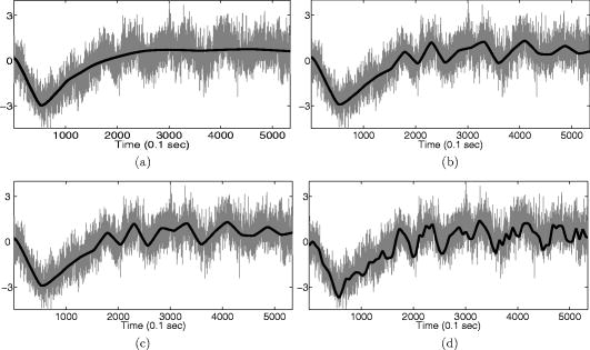
Recall that the $α$ value in the AR(1) model denotes the degree of correlation between the neighborhood samples. Even though this paper chose $α = 0.8$ to represent relatively strong correlation between the neighboring samples, similar behaviors have been obtained for a wide range of $α$ values, and our Wavelet-MDL framework has been observed to outperform the other methods for all cases.

5.2.

Experimental NIRS Data

We now apply our algorithm to real NIRS measurements. For calculating $t$ -values, we used NIRS-SPM software, which has been developed by our group.¹¹ NIRS-SPM allows the estimation of the temporal correlation and determines a $p$ -value using the tube formula. For a detailed discussion on the estimation of the temporal correlation, $p$ -value, and related threshold value, readers can refer to our previous work on this issue.¹¹ In NIRS-SPM, the conventional filtering based on DCT is implemented. We set the cutoff frequency as $1 ∕ 60 Hz$ , which is below the frequency of RFT paradigm repetition frequency of $0.018 Hz$ .

In Fig. 4a, the deoxy-hemoglobin (HbR) $t$ -map from NIRS-SPM using Wavelet-MDL is illustrated. For clear comparison, the magnified figure is illustrated in Fig. 4b, whereas Fig. 4c shows the result of the conventional DCT filtering approach. The temporal covariance was estimated using a prewhitening method.¹¹ While the task-related activation is observable in both cases, Wavelet-MDL provides a higher $t$ -value centered at the target area. The maximum $t$ -values were 13.95 and 13.16 for Wavelet-MDL and the DCT-based filtering, respectively. The higher $t$ -values indicate that the proposed method provides a statistically more significant estimate of the activation map.

Fig. 4

Deoxyhemoglobin $t$ -maps for the RFT experiment. (a) Result from NIRS-SPM. Magnified $t$ -maps using (b) Wavelet-MDL and (c) the conventional method. The wavelet-MDL detrending method provides a higher $t$ -value centered at the target area.

An oxyhemoglobin time series and trend estimates are illustrated in Fig. 5 . Since the design matrix is explicitly incorporated during the detrending process of Wavelet-MDL, as described in Eq. 20, the oxyhemoglobin signals were almost conserved, as shown in Fig. 5a. However, in the case of the conventional approach, some components of oxyhemoglobin signals were classified as global trends, as illustrated in Fig. 5b. Figure 6 shows another oxyhemoglobin signal that contains a rapidly varying bias. If we use the conventional detrending method, the residual of the fast-varying transient trend can be classified as an oxyhemoglobin signal. However, Wavelet-MDL can estimate the unknown trend even if it has high-frequency transient signal, since it is capable of capturing the transient signal and adjusting the complexity of a global trend automatically, as illustrated in Fig 6a. However, in Fig. 6b, the fast varying trend was not fully captured by the conventional approach, and the hemodynamic signal was damaged.

Fig. 5

Oxyhemoglobin measurement during the RFT experiment and estimated trend with (a) Wavelet-MDL and (b) the conventional method. The task-related signals are not removed for the case of Wavelet-MDL.

Fig. 6

Oxyhemoglobin measurement during the RFT experiment and estimated trend with (a) Wavelet-MDL and (b) the conventional method. Wavelet-MDL is capable of removing fast-varying trends without damaging task-related signals.

Last, we compared MDL with ${AIC}_{C}$ , SIC, and Saito’s MDL. Figures 7b, 7c, 7d show that the estimated trends based on ${AIC}_{C}$ , SIC, and Saito’s MDL result in overfitting, whereas our algorithm correctly captures the trends. This implies that the modified universal prior of the integer is effective in model order selection.

Fig. 7

Trend estimate using (a) the proposed MDL, (b) Saito’s MDL, (c) SIC, and (d) ${AIC}_{C}$ . Compared with other model order criteria, the proposed method gives the most accurate estimate.

5.3.

Group Analysis

Group analyses were performed using NIRS-SPM software. NIRS data as well as simultaneously recorded fMRI data from nine subjects were used. Figure 8 shows group activation maps for the HbR signal at $p = 0.05$ , which is overlayed on the fMRI activation map at $p = 0.005$ . The Wavelet-MDL detrending method gives more specific localization of the target motor cortex compared to the conventional DCT-based high-pass filtering. To quantify the accuracy of localization, we calculate the receiver operating characteristic (ROC) for the spatial correlation of the NIRS activation map with that of fMRI BOLD. An ROC curve is a graphical plot of “sensitivity” versus “1-specificity” for a binary classifier. In ROC, (0,1) is the point of an ideal classifier, and the diagonal line represents the performance of random guessing. Therefore, the area under the ROC curve is a good indicator of the performance of a classifier. We evaluated our detrending method by measuring the spatial correlation between NIRS activation maps and the fMRI BOLD map. The BOLD map with $p = 0.005$ was assumed as the ground truth in Fig. 9 . The sensitivity and specificity were calculated by changing the threshold values. The ROC analysis in Fig. 9 shows that the proposed detrending algorithm outperforms the conventional high-pass filtering since the area under the ROC curve is largest for Wavelet-MDL.

Fig. 8

NIRS-SPM group analysis result at $p = 0.05$ . (a) Wavelet-MDL detrending and (b) DCT based detrending. Wavelet-MDL provides a more specific activation map. The mesh image corresponds to the fMRI activation map at 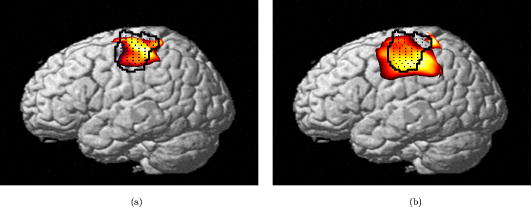$p = 0.005$ .

Fig. 9

ROC curves for activation maps using Wavelet-MDL and DCT-based detrending. The fMRI activation map at $p = 0.005$ shown as an inset is used as a ground truth, and the sensitivity and the specificity were calculated by changing the threshold value. The ROC analysis shows that the area under the ROC curve for Wavelet-MDL was largest, indicating that the proposed algorithm outperforms the conventional method.

6. Discussion

6.1.

Temporal Covariance in MDL

In Eq. 26, we assume that the noise is uncorrelated, independent, and normally distributed. For the correlated noise, the covariance matrix $Σ$ should be considered in Eqs. 26, 27, 28. Specifically, consider the negative log-likelihood for measurement in the wavelet domain. Let $r (n_{0})$ denote the residual vector for model order $n_{0}$ in the wavelet domain, i.e., $r (n_{0}) = W (y - X β - θ)$ . Since the dependency for $r$ on the model order $n_{0}$ is clear in the context, we omit the letter $n_{0}$ in the sequel. If we model the correlated noise using the fractional Brownian motion process²⁶ as in the fMRI case,¹⁶ the pdf of measurement $y$ in the wavelet domain is given by

Eq. 37

p (W y ∣ n_{0}) = \frac{1}{{(2 π)}^{2 N} {∣ Σ ∣}^{1 ∕ 2}} \exp (- \frac{1}{2} r^{T} Σ^{- 1} r),

where

Σ

denotes a diagonal covariance matrix described in Eq. 22. If we substitute Eq. 22 for

Σ

in Eq. 37, the negative log-likelihood for measurement is then given by

Eq. 38

- \log p (W y ∣ n_{0}) = \frac{1}{2} \sum_{j = 1}^{J} [N_{j} \log σ_{j}^{2} (n_{0}) + σ_{j}^{- 2} (n_{0}) r_{j}^{T} r_{j}] + c,

where

N_{j} = 2^{- j} N

is the number of wavelet coefficients in the

j

’th scale,

r_{j}

is the subvector of

r

corresponding to the

j

’th scale, and

c

is a constant not related to model order selection. The maximum likelihood (ML) estimator for level-dependent variance

σ_{j}^{2} (n_{0})

is easily obtained by a straightforward calculation as follows:

Eq. 39

{\hat{σ}}_{j}^{2} (n_{0}) = \frac{1}{N_{j}} r_{j}^{T} r_{j},

which is identical with the ML estimates of the residual variance in the

j

’th scale. If we substitute Eq. 39 for

σ_{j}^{2} (n_{0})

in Eq. 38:

Eq. 40

- \log p (W y ∣ n_{0}) = \sum_{j = 1}^{J} \frac{N_{j}}{2} \log {\hat{σ}}_{j}^{2} (n_{0}) + c^{″},

where

c^{″}

is a constant not related to model order selection. Now, we employ an exponentially decaying variance model along decomposition levels that is popularly used for modeling the correlated noise in the wavelet domain:^{24, 45, 46}

Eq. 41

σ_{j}^{2} (n_{0}) = τ^{2} (n_{0}) 2^{α j},

where

α

is the spectral decay rate of the correlated noise model and

τ

denotes a constant that reflects the overall noise variance. We can estimated

τ

in the zeroth, decomposition level, i.e., in the time domain, as follows:

Eq. 42

{\hat{τ}}^{2} (n_{0}) = {\hat{σ}}_{0}^{2} (n_{0}) = \frac{1}{N} {‖ y - X β - θ (n_{0}) ‖}^{2} .

By substituting Eq. 41 and Eq. 42 for

{\hat{σ}}_{j}^{2} (n_{0})

in Eq. 40, we obtain

Eq. 43

- \log p (W y ∣ n_{0}) = \frac{N}{2} \log {\hat{σ}}_{0}^{2} (n_{0}) + c^{‴},

where

c^{‴}

is a constant not related to model order selection. Hence, Eq. 43 is identical to Eq. 28.

6.2.

$t$ -Value versus Activation Map

Recall that $t$ -value is often used to quantify the performance of the detrending algorithms.¹⁶ However, more correct quantification should be based on the accuracy of the activation map at the same $p$ -value. For example, consider a case where a fixed $p$ -value provides an identical threshold value. Then, in obtaining the activation maps, the overall increase in $t$ -values may imply that the resulting activation map becomes significantly larger. Hence, to guarantee the accurate localization, the higher contrast of $t$ -value between activated and background region is more important. In this perspective, our group analysis result confirms that wavelet-MDL detrending is more accurate in localizing the activation maps.

6.3.

Precoloring versus Prewhitening

In Ref. 11, we have proposed two different methods to remove the temporal covariance: precoloring and prewhitening. Precoloring tries to remove the temporal correlation by filtering with HRF filter, whereas prewhitening attempts to estimate $Σ$ based on the assumption that the noise is the AR(1) process. In this perspective, the prewhitening provides more accurate estimation of $Σ$ as long as the AR(1) assumption is correct. The $t$ -value in Fig. 4 was hence calculated using prewhitening. However, as demonstrated in Ref. 11, precoloring was more robust in removing the temporal correlation, and the final activation maps from precoloring were observed to be better due to the limited number of measurements compared to its fMRI counterpart.¹¹ Hence, this paper calculates the group activation map using the precoloring method, as in. Ref. 11.

7. Conclusion

We developed a Wavelet-MDL-based detrending method that is robust under motion and physiological variation. In Wavelet-MDL detrending, a wavelet transform is applied to the NIRS time series to decompose it into bias, hemodynamic signal, and noise components in distinct scales. With the MDL criterion using a modified universal prior for the integer, the optimal model order could be easily estimated, and the unknown drift signal in NIRS data was successfully removed. Experimental results demonstrated that the new detrending algorithm outperforms the conventional approaches.

Acknowledgments

This work was supported by the IT R&D program of MKE/IITA [2008-F-021-01]. K. E. Jang gratefully acknowledges support from a Kim Bo Jung Scholarship. K. E. Jang is currently at Samsung Advanced Institute of Technology.

References

1.

F. F. Jobsis, “Noninvasive, infrared monitoring of cerebral and myocardial oxygen sufficiency and circulatory parameters,” Science, 198 1264 –1267 (1977). https://doi.org/10.1126/science.929199 0036-8075 Google Scholar

2.

S. G. Diamond, T. J. Huppert, V. Kolehmainen, M. A. Franceschini, J. P. Kaipio, S. R. Arridge, and D. A. Boas, “Dynamic physiological modeling for functional diffuse optical tomography,” Neuroimage, 30 (1), 88 –101 (2006). https://doi.org/10.1016/j.neuroimage.2005.09.016 1053-8119 Google Scholar

3.

Y. Hoshi, “Functional near-infrared optical imaging: utility and limitations in human brain mapping,” Psychophysiology, 40 511 –520 (2003). https://doi.org/10.1111/1469-8986.00053 0048-5772 Google Scholar

4.

M. Cope and D. T. Delpy, “System for long-term measurement of cerebral blood and tissue oxygenation on newborn infants by near infra-red transillumination,” Med. Biol. Eng. Comput., 26 289 –294 (1988). https://doi.org/10.1007/BF02447083 0140-0118 Google Scholar

5.

M. Essenpreis, M. Cope, C. E. Elwell, S. R. Arridge, P. van der Zee, and D. T. Delpy, “Wavelength dependence of the differential pathlength factor and the log slope in time-resolved tissue spectroscopy,” Adv. Exp. Med. Biol., 333 9 –20 (1993). 0065-2598 Google Scholar

6.

A. Duncan, J. H. Meek, M. Clemence, C. E. Elwell, L. Tyszczuk, M. Cope, and D. T. Delpy, “Optical pathlength measurements on adult head, calf, and forearm and the head of the newborn infant using phase resolved optical spectroscopy,” Phys. Med. Biol., 40 295 –304 (1995). https://doi.org/10.1088/0031-9155/40/2/007 0031-9155 Google Scholar

7.

H. Zhao, Y. Tanikawa, F. Gao, Y. Onodera, A. Sassaroli, K. Tanaka, and Y. Yamada, “Maps of optical differential pathlength factor of human adult forehead, somatosensory motor, and occipital regions at multi-wavelengths in NIR,” Phys. Med. Biol., 47 (12), 2075 –2093 (2002). https://doi.org/10.1088/0031-9155/47/12/306 0031-9155 Google Scholar

8.

M. L. Schroeter, M. M. Bucheler, K. Muller, K. Uludag, H. Obrig, G. Lohmann, M. Tittgemeyer, A. Villringer, and D. Yves von Cramon, “Towards a standard analysis for functional near-infrared imaging,” Neuroimage, 21 283 –290 (2004). https://doi.org/10.1016/j.neuroimage.2003.09.054 1053-8119 Google Scholar

9.

M. M. Plichta, S. Heinzel, A. C. Ehlis, P. Pauli, and A. J. Fallgatter, “Model-based analysis of rapid event-related functional near-infrared spectroscopy (NIRS) data: a parametric validation study,” Neuroimage, 35 625 –634 (2007). https://doi.org/10.1016/j.neuroimage.2006.11.028 1053-8119 Google Scholar

10.

P. H. Koh, D. E. Glaser, G. Flandin, S. Kiebel, B. Butterworth, A. Maki, D. T. Delpy, and C. E. Elwell, “Functional optical signal analysis: a software tool for near-infrared spectroscopy data processing incorporating statistical parametric mapping,” J. Biomed. Opt., 12 1 –13 (2007). https://doi.org/10.1117/1.2804092 1083-3668 Google Scholar

11.

J. C. Ye, S. Tak, K. E. Jang, J. Jung, and J. Jang, “NIRS-SPM: statistical parametric mapping for near-infrared spectroscopy,” Neuroimage, 44 (2), 428 –447 (2009). https://doi.org/10.1016/j.neuroimage.2008.08.036 1053-8119 Google Scholar

12.

K. J. Worsley and K. J. Friston, “Analysis of fMRI time-series: revisited again,” Neuroimage, 2 173 –181 (1995). https://doi.org/10.1006/nimg.1995.1023 1053-8119 Google Scholar

13.

J. Sun, “Tail probabilities of the maxima of Gaussian random fields,” Ann. Probab., 21 (1), 34 –71 (1993). https://doi.org/10.1214/aop/1176989393 0091-1798 Google Scholar

14.

J. Cao and K. J. Worsley, “The geometry of the Hotellings random field with applications to the detection of shape changes,” Ann. Stat., 27 (3), 925 –942 (1999). https://doi.org/10.1214/aos/1018031263 0090-5364 Google Scholar

15.

Statistical Parametric Mapping: The Analysis of Functional Brain Images, Academic Press, San Diego, CA (2006). Google Scholar

16.

F. G. Meyer, “Wavelet-based estimation of a semiparametric generalized linear model of fMRI time-series,” IEEE Trans. Med. Imaging, 22 (3), 315 –322 (2003). https://doi.org/10.1109/TMI.2003.809587 0278-0062 Google Scholar

17.

J. Rissanen, “Modeling by shortest data description,” Automatica, 14 (5), 465 –471 (1978). 0005-1098 Google Scholar

18.

K. J. Friston, A. P. Holmes, K. J. Worsley, J.-P. Poline, C. D. Frith, and R. S. J. Frackowiak, “Statistical parametric maps in functional imaging: a general linear approach,” Hum. Brain Mapp, 2 (4), 189 –210 (1995). https://doi.org/10.1002/hbm.460020402 1065-9471 Google Scholar

19.

R. W. Cox, “AFNI: software for analysis and visualization of functional magnetic resonance neuroimages,” Comput. Biomed. Res., 29 162 –173 (1996). https://doi.org/10.1006/cbmr.1996.0014 0010-4809 Google Scholar

20.

G. M. Boynton, S. A. Engel, G. H. Glover, and D. J. Heeger, “Linear systems analysis of functional magnetic resonance imaging in human V1,” J. Neurosci., 16 4207 –4221 (1996). 0270-6474 Google Scholar

21.

R. N. A. Henson, C. J. Price, M. D. Rugg, R. Turner, and K. J. Friston, “Detecting latency differences in event-related BOLD responses: application to words versus nonwords and initial versus repeated face presentations,” Neuroimage, 15 83 –97 (2002). https://doi.org/10.1006/nimg.2001.0940 1053-8119 Google Scholar

22.

S. G. Mallat, A Wavelet Tour of Signal Processing, Academic, New York (1999). Google Scholar

23.

I. M. Johnstone and B. W. Silverman, “Wavelet threshold estimators for data with correlated noise,” J. R. Stat. Soc. Ser. B (Methodol.), 59 (2), 319 –351 (1997). https://doi.org/10.1111/1467-9868.00071 0035-9246 Google Scholar

24.

P. Flandrin, “Wavelet analysis and synthesis of fractional Brownian motion,” IEEE Trans. Inf. Theory, 38 (2), 910 –917 (1992). https://doi.org/10.1109/18.119751 0018-9448 Google Scholar

25.

D. Ville, M. L. Seghier, F. Lazeyras, T. Blu, and M. Unser, “WSPM: wavelet-based statistical parametric mapping,” Neuroimage, 37 (4), 1205 –1217 (2007). https://doi.org/10.1016/j.neuroimage.2007.06.011 1053-8119 Google Scholar

26.

B. B. Mandelbrot and J. W. Ness, “Fractional Brownian motions, fractional noises, and applications,” SIAM Rev., 10 (4), 422 –437 (1968). https://doi.org/10.1137/1010093 0036-1445 Google Scholar

27.

D. Donoho and I. M. Johnstone, “Ideal spatial adaptation by wavelet shrinkage,” Biometrika, 81 (3), 425 –455 (1994). https://doi.org/10.1093/biomet/81.3.425 0006-3444 Google Scholar

28.

N. Saito, “Simultaneous noise suppression and signal compression using a library of orthonormal bases and the minimum description length criterion,” Wavelets Geophys., 299 –324 1994). Google Scholar

29.

J. Rissanen, “MDL denoising,” IEEE Trans. Inf. Theory, 46 (7), 2537 –2543 (2000). https://doi.org/10.1109/18.887861 0018-9448 Google Scholar

30.

K. J. Friston, P. Fletcher, O. Josephs, A. Holmes, M. D. Rugg, and R. Turner, “Event-related fMRI: characterizing differential responses,” Neuroimage, 7 30 –40 (1998). https://doi.org/10.1006/nimg.1997.0306 1053-8119 Google Scholar

31.

K. L. Hurvich and C. L. Tsai, “Regression and time series model selection in small samples,” Biometrika, 76 (2), 297 –307 (1989). https://doi.org/10.1093/biomet/76.2.297 0006-3444 Google Scholar

32.

G. Schwarz, “Estimating the dimension of a model,” Ann. Stat., 6 461 –464 (1978). https://doi.org/10.1214/aos/1176344136 0090-5364 Google Scholar

33.

H. Akaike, “A new look at the statistical model identification,” IEEE Trans. Autom. Control, AC-19 (6), 716 –723 (1974). https://doi.org/10.1109/TAC.1974.1100705 0018-9286 Google Scholar

34.

S. Kullback and R. A. Leibler, “On information and sufficiency,” Ann. Math. Stat., 22 (1), 79 –86 (1951). https://doi.org/10.1214/aoms/1177729694 0003-4851 Google Scholar

35.

P. Stoica and Y. Selen, “Model-order selection: a review of information criterion rules,” IEEE Signal Process. Mag., 21 36 –47 (2004). https://doi.org/10.1109/MSP.2004.1311138 1053-5888 Google Scholar

36.

A. Kolmogorov, “Three approaches to the quantitative definition of information,” Probl. Inf. Transm., 1 4 –7 (1965). 0032-9460 Google Scholar

37.

T. Cover and J. A. Thomas, Elements of Information Theory, 2nd ed.John Wiley & Sons, Inc., New York (1991). Google Scholar

38.

M. Hansen and B. Yu, “Model selection and the principle of minimum description length,” J. Am. Stat. Assoc., 96 (454), 746 –774 (2001). https://doi.org/10.1198/016214501753168398 0162-1459 Google Scholar

39.

J. Rissanen, “A universal prior for integers and estimation by minimum description length,” Ann. Stat., 11 (2), 417 –431 (1983). https://doi.org/10.1214/aos/1176346150 0090-5364 Google Scholar

40.

M. Unser, “A practical guide to the implementation of the wavelet transform,” Wavelets in Medicine and Biology, 37 –73 1996). Google Scholar

41.

A. Cohen, I. Daubeches, and J. C. Feauveau, “Biorthogonal bases of compactly supported wavelets,” Commun. Pure Appl. Math., 45 (5), 485 –560 (1992). https://doi.org/10.1002/cpa.3160450502 0010-3640 Google Scholar

42.

B. E. Usevitch, “A tutorial on modern lossy wavelet image compression: foundations of JPEG 2000,” IEEE Signal Process. Mag., 18 (5), 22 –35 (2001). https://doi.org/10.1109/79.952803 1053-5888 Google Scholar

43.

A. V. Oppenheim and R. W. Schafer, Discrete-Time Signal Processing, Prentice Hall, Upper Saddle River, NJ (1989). Google Scholar

44.

P. L. Purdon and R. M. Weisskoff, “Effect of temporal autocorrelation due to physiological noise and stimulus paradigm on voxel-level false-positive rates in fMRI,” Hum. Brain Mapp, 6 (4), 239—249 (1998). https://doi.org/10.1002/(SICI)1097-0193(1998)6:4<239::AID-HBM4>3.0.CO;2-4 1065-9471 Google Scholar

45.

E. Bullmore, C. Long, J. Suckling, J. Fadili, G. Calvert, F. Zelaya, T. A. Carpenter, and M. Brammer, “Colored noise and computational inference in neurophysiological (fMRI) time series analysis: resampling methods in time and wavelet domains,” Hum. Brain Mapp, 12 (2), 61 –78 (2001). https://doi.org/10.1002/1097-0193(200102)12:2<61::AID-HBM1004>3.0.CO;2-W 1065-9471 Google Scholar

46.

J. M. Fadili and E. Bullmore, “Penalized partially linear models using sparse representations with an application to fMRI time series,” IEEE Trans. Signal Process., 53 (9), 3436 –3448 (2005). https://doi.org/10.1109/TSP.2005.853207 1053-587X Google Scholar

Citation Download Citation

Kwang-Eun Jang, Sungho Tak, Jinwook Jung, Jaeduck Jang, Yong Jeong, and Yong Chul Ye "Wavelet minimum description length detrending for near-infrared spectroscopy," Journal of Biomedical Optics 14(3), 034004 (1 May 2009). https://doi.org/10.1117/1.3127204

Published: 1 May 2009

Access the abstract

JOURNAL ARTICLE
13 PAGES

DOWNLOAD PAPER SAVE TO MY LIBRARY