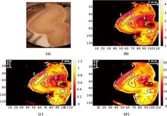
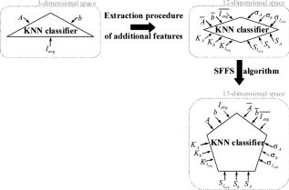
2.1.

Tissue Scatter Imaging

The scatter imaging system consisted of a weakly confocal spectroscopic system having illumination and detection spot sizes smaller than one mean scattering length (typically, $100\mu \mathrm{m}$ for tissue¹³), and a raster-scanning platform built using linear translation stages. This spot size was specifically chosen because it provides a scatter signal that does not have significant contributions from multiple scattering, making it essentially linearly dependent on the scatter coefficient. The instrument operates in the $510–785\mathrm{nm}$ spectral waveband with a broadband fiber-coupled tungsten-halogen light source. An optical-fiber coupled to a CCD-based spectrometer was used for confocal spectroscopic detection, with a spectral resolution of $\sim 1\mathrm{nm}$ . All spectral measurements were referenced to a Spectralon-based reflectance standard, which removes instrumental spectral response from the sample measurements and allows direct comparisons of the extracted scatter parameters across different samples. Average sample scanning time was $\sim 1\mathrm{h}$ , mainly due to the use of mechanical stages for raster scanning. Sufficient precautions were taken to prevent the sample from drying during the measurement sequence. A schematic and a more detailed description of the system can be found in a previous paper.⁶

In the presence of significant local absorption, for very small source-detector separations, the spectral reflectance can be estimated by an empirical relationship as follows:

Human pancreatic tumor cells ASPC-1 were grown and injected subcutaneously in the flank region of male mice. Tumors were harvested seven weeks after injection when they measured $6–7\mathrm{mm}$ in diameter and $5–6\mathrm{mm}$ in thickness. Then they were dissected into $4–5\mathrm{mm}$ thick sections and imaged using the mentioned scatter imaging system. In total, six tumor tissue sections harvested from four mice were imaged. After the measurement, the sample was routinely processed for histology evaluation by paraffin embedding, $4\mu \mathrm{m}$ sectioning and H&E staining.⁶ The top full-view slide from each sample was used for pathologic analysis. A veterinary pathologist examined the H&E slides from each sample and identified several regions-of-interest corresponding to the observed tissue subtypes. These were classified under three major groups, namely, epithelium, fibrosis, and necrosis, with constituent subgroups: two distinct types of epithelial cells, according to the exhibited nucleus to cytoplasm ratio, were considered (low and high proliferation index) and regions exhibiting fibrosis were classified into early, intermediate, and mature fibrosis subgroups. Figure 1 shows an example of a pancreas tumor sample, where five regions of interest are shown overlaid on the scattered amplitude $A$ , scattering power $b$ , and average scattered irradiance $I_{\mathrm{avg}}$ images. Color bar scales of the scattering parameters are shown on the right of their corresponding images. Region 1 shows LPI tumor cells with less cellular density compared to HPI tumor cells found in region 2. Region 3 shows necrosis, and regions 4 and 5 show the early and intermediate stages of fibrosis, respectively. Apart from the tumor tissue samples mentioned above, $3–4\text{-}\mathrm{mm}$ -thick tissue sections of normal pancreas were harvested from three male mice and were imaged using the scatter imaging system.

Fig. 1

(b) Scattered amplitude, $A$ ; (c) scattering power, $b$ ; and (d) average scattered irradiance, $I_{\mathrm{avg}}$ images of a pancreas tumor sample (a) showing five pathology-based regions of interest overlaid on it.

2.2.

Classification Methods

2.2.1.

$K$ -nearest neighbors

The $K$ -nearest neighbor (KNN) classifier¹⁷ consisted in the assignment of an unclassified vector using the $\mathit{k}$ closest vectors found in the training set. This approach can naturally deal with multiclass data while some of the more advanced classifiers, such as support vector machines (SVM),¹⁸ require the bridging of results from a combinatorial set of such classifiers to simulate multiclass parameters.¹⁹ Using the KNN classifier, both normal versus tumor sample segmentation and the discrimination of pathologically distinct tumor regions were performed using the same methodology.

A schematic of the KNN process for classifying normal versus tumor tissue using three independent scatter-related parameters is depicted in Fig. 2 . The map was populated by points, each of which represents a tissue pixel with its own set of scattering parameters. Every pixel inside the predefined regions of interest was considered as a vector in a three-dimensional space (hereinafter called feature space), and it was plotted in the map using the three numerical values of its scattering parameters as the $x,y,z$ coordinate values. Because KNN is based on considering that similar data values should belong to the same class or region, the normal tissue or tumor in this case, then $K$ pixels with the most similar scattering parameters to an unclassified pixel were initially determined. This similarity was estimated in terms of the Euclidean distance

Eq. 2

$D(p_1,p_2)=\sqrt{{(A_1-A_2)}^2+{(b_1-b_2)}^2+{(I_{\mathrm{avg}1}-I_{\mathrm{avg}2})}^2},$

where $p_1$ and $p_2$ are the two compared tissue pixel localizations, and $A$ , $b$ and $I_{\mathrm{avg}}$ stand for their scattering amplitude, scattering power, and average scattered irradiance, respectively. The unclassified pixel will be assigned to the most numerous tissue type (normal or tumor) among the $K$ closest neighbors. Therefore, this classifier has only one independent parameter, $K$ or the number of neighbors, to consider. In the proposed methodology, different values of the parameter $K$ are evaluated. Figure 3 shows in more detail how the KNN classifier works for a fixed value of parameter $K$ $(K=10)$ . The unknown black tissue pixel localization needs to be assigned either to tumor or normal tissue classes, depicted with triangles and circles, respectively. The first step is to determine the nearest ten $(K=10)$ neighbors as given by Eq. 2. The resulting ten pixel localizations are the ones surrounded by the red circle. As seven pixels out of ten are normal tissue and only three pixels are tumor, the outcome of the KNN classifier indicates that the unknown pixel corresponds to normal tissue.

Fig. 2

Schematic of the normal versus tumor discrimination by means of the KNN classifier, where the three measurement parameters are each considered a coordinate axis and the distance between points in this Cartesian space then defines how similar or different they are.

Fig. 3

Example of pixel tissue-type determination $(K=10)$ .

Because KNN is based on distances between sample points in the feature space, all parameters need to be normalized to prevent some features being more strongly weighted than others.¹⁹ Hence, all the three scattering parameters were unity normalized by the mean, before the classification process.

Segmentation of pathologically distinct tumor regions by means of the KNN classifier was similar to the normal versus tumor classification described above, except for the fact that there were six different classes (low proliferation index and high proliferation index epithelium, necrosis, early, intermediate and mature fibrosis) and the unknown pixel was assigned to the most numerous class among these six.

2.2.2.

Additional statistical data for the KNN classification

As the number of features in a data set varies from 1 to $\infty$ , any classifier accuracy rises to a maximum and then falls back asymptotically.²⁰ In the segmentation of the tumor regions, the six different tissue morphologies mentioned above have to be discriminated from a data set that lies in a three-dimensional space. Therefore, an additional feature extraction from the actual data set is required to decrease the discrimination error. In Ref. 19 a three-step automated breast-tissue classification methodology is proposed. The breast area is first segmented into fatty versus dense mammographic tissue, and the second step precisely consists of the extraction of morphological features by means of statistics calculations within the previously segmented breast areas. Because segmentation does not apply here (because that is the aim of the proposed methodology), a square spatial vicinity centered in each pixel location is defined. Then the first four statistical moments (mean, standard deviation, skewness, and kurtosis) of each scattering parameter are computed inside that vicinity region. Statistics are either concatenated with the fitted scattering parameters themselves or can be used on their own to form higher dimensional feature spaces. This procedure is graphically described in Fig. 4 . Initially, each data point lies in a three-dimensional space (the $A-b-I_{\mathrm{avg}}$ space). Then the statistical moments of each point are estimated inside a moving window centered in the pixel of interest. These moments on their own form a 12-dimensional space, whereas if they are concatenated with the three input parameters, each data point becomes a vector in a 15-dimensional space. The third and forth moments, the skewness, and the kurtosis, respectively, measure the bias and the probability of outlier occurrence, respectively, of each scattering parameter distribution inside the defined window. The behavior of the methodology in terms of the classification error is studied as a function of the number of neighbors but also as a function of the window size, where the latter is defined as the side length of the squared vicinity region. The study of KNN classification was completed with all the parameters for varying spatial window sizes, and an optimal window size was used for the final process.

Fig. 4

Block diagram of higher dimensional space constructions and classification procedure.

In addition, a further study on the capability of both the scattering parameters and their extracted statistics (mean, standard deviation, skewness, and kurtosis) to discriminate the different tumor regions was then performed. In this study, the sequential floating forward selection (SFFS) algorithm²¹ was used because it is widely applied to reduce the dimensionality (i.e., the number of features) of spectral data prior to interpretation.^{22, 23} When processing spectral data, the feature calculates mean values at each one of the spectral bands and the aim of SFFS in this case is to select the $M$ spectral bands that best discriminate among the subject classes, out of the total number $N$ initial bands, so $M<N$ . The discrimination among the classes, or class separability, can be calculated performing different statistical computations.²² The same fundamental is employed to sort the scattering parameters and their statistical values according to their subtype discrimination capability. In this way, the first feature selected by the algorithm will be the one with the greatest changes according to the pathology. As in Ref. 22, the Bhattacharya statistical distance was employed to measure these changes. Therefore, the difference in a scattering parameter $p$ , with $p=1,2,\dots ,15$ , between two tissue subtypes, $i$ and $j$ , is given by

Eq. 3

$J_{ij}^p=\frac{1}{4}{({\mu }_j-{\mu }_i)}^T{[{\Sigma }_i+{\Sigma }_j]}^{-1}({\mu }_j-{\mu }_i)+\frac{1}{2}\ln \left(\frac{\mid {\Sigma }_i+{\Sigma }_j\mid }{2{(\mid {\Sigma }_i\mid \cdot \mid {\Sigma }_j\mid )}^{1∕2}}\right),$

where ${\mu }_i$ and ${\sum }_i$ are the mean and the variance matrix of $p$ for tissue subtype $i$ . Because there are six different tissue subtypes, the globlal class separability measurement, $J$ , requires one to calculate the difference between every two subtypes

Eq. 4

$J=\sum _{i=1}^6\sum _{j=i+1}^6{P}_i{P}_j{J}_{ij},$

where $P_i$ is each subtype probability and $J_{ij}$ is the distance between subtypes $i$ and $j$ , as stated in Eq. 4.

2.3.

Quantitative Evaluation of Tissue Discrimination Capability

In order to accurately estimate the performance of the discrimination methodology a threefold cross-validation technique or procedure^{24, 25} was applied both in the tumor versus normal and tumor region discrimination. A total of $\mathrm{16,599}\text{pixels}$ within the regions of interest of three normal samples and $3660\text{pixels}$ within the regions of interest of five tumor samples were considered. This data set was divided into three nonoverlapping sets containing 6653 data points each (5533 of normal tissue and 1120 of tumor). Two of these sets were employed as the training set, and the other one, the so-called validation set, was used to calculate the error of the classifier. The latter is mathematically given by

Pixels corresponding to locations where the scatter data could not be reliably measured were tagged as masked pixels. These pixels were neither included in the training nor the validation sets of the cross-validation procedure.

3.1.

Tumor versus Normal Tissue Discrimination

Figure 5 shows the actual three-dimensional map representing the pixel locations in the $A\text{-}b\text{-}{I}_{\mathrm{avg}}$ space [Fig. 5a] and its three corresponding two-dimensional maps: $A$ versus $I_{\mathrm{avg}}$ [Fig. 5b] $A$ versus $b$ [Fig. 5c] and $b$ versus $I_{\mathrm{avg}}$ [Fig. 5d]. Normal pixels appear well grouped, whereas a remarkable spreading is observed in the scattering parameters of tumor pixels.

Fig. 5

Grouped scatter plots for normal and tumor pixel localizations in the three input data parameters, $A-b-I_{\mathrm{avg}}$ , (a) space and (b–d) its corresponding two-dimensional spaces.

Figure 6 depicts the behavior of the KNN algorithm in the discrimination of normal and tumor tissue pixel locations as a function of the number of considered neighbors. Classification accuracy should be expected to increase with the number of neighbors because this reduces the influence of outliers (i.e., training data points assigned to a wrong class). There were no outliers here because the distinct sample regions were segmented as indicated by the pathologist. This absence of outliers, together with the spreading of tumor scattering parameters, caused an increase in the classification error percentage with the number of neighbors. This influence of the scattering parameter spreading on classification has been proved, employing as training set those pixels whose scattering parameters are close to the mean of each parameter and an independency of error probability on the number of neighbors has been obtained. Finally, discrimination results for all pixel locations in both normal and tumor samples, while considering only one neighbor, are presented in Figs. 7 and 8 . An absolute correlation was achieved between automatic and expert-based classification within the predefined regions of interest. In fact, the three normal samples in Fig. 7 were entirely correctly classified as well as the four tumor samples in Fig. 8. Only some errors are encountered within the regions of interest in the fifth tumor sample. A quantitative measurement of tissue-type discrimination, including percentages of pixels lost as masked pixels (inside the samples) and number of correctly identified localizations per sample is presented in Table 1 . Tissue discrimination capability of the approach is, however, measured in terms of the quantities presented in Fig. 6 because they are obtained through the cross-validation procedure described before, which removes the dependency of classification results on the training or test sets.

Fig. 6

Behavior of the methodology in normal versus tumor discrimination when the number of considered neighbors increases.

Fig. 7

Normal and tumor pixel discrimination in normal samples using the three scatter measured parameters.

Fig. 8

Normal and tumor pixel discrimination in tumor samples using the three scatter measured parameters.

Table 1

Quantitative measurement of tissue-type discrimination.

3.2.

Segmentation of Pathologically Distinct Tumor Regions

Figure 9 depicts some pixel localizations of the tumor samples in the $A\text{-}b\text{-}{I}_{\mathrm{avg}}$ space [Fig. 9a] and its three corresponding two-dimensional maps: $A$ versus $I_{\mathrm{avg}}$ [Fig. 9b], $A$ versus $b$ [Fig. 9c] and $b$ versus $I_{\mathrm{avg}}$ [Fig. 9d]. For visualization purposes only, those tumor pixels whose scattering parameters were within the interval $p∊[\overline{p}-{\sigma }_p∕3,\overline{p}+{\sigma }_p∕3]$ , where $p$ is each of the three scattering parameters and $\overline{p}$ and ${\sigma }_p$ are respectively its mean and variance, are represented in the map. As expected, because of the subtle changes in the scattering parameters, pixel localizations do not appear well grouped according to their tissue subtype. The behavior of the KNN methodology in the discrimination of these pathologically distinct tumor regions as a function of the number of neighbors is shown in Fig. 10, where an increase in the classification error percentage occurs as the number of neighbors grows. Figure 11 displays the segmentation of the different regions in tumor samples by means of the KNN with $K=1$ , while Table 2 summarizes the same information as a confusion matrix, where each row represent the total number of pixel localizations in each tumor subtype (as defined by the pathologist inside the regions of interest). It seems that the automated classification accurately imitates the regions-of-interest identification process performed by the pathologist. However, once generality on the training and test sets is attained by means of the cross-validation procedure, an $\sim 9\%$ classification error occurs within these regions of interest, as shown in Fig. 10. Statistical data, as described in Sec. 2.2, was added to improve the performance of the methodology.

Fig. 9

Grouped scatter plots for all tumor sub-types in the $A-b-I_{\mathrm{avg}}$ (a) space and (b–d) its corresponding two-dimensional spaces.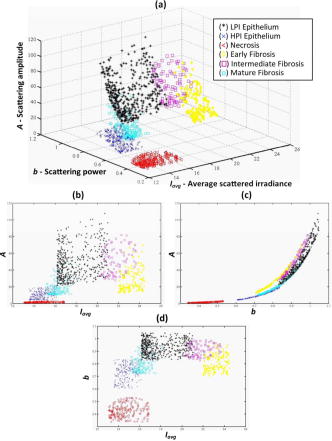

Fig. 10

Behavior of the KNN methodology in tumor subtype discrimination as a function of the number of neighbors.

Fig. 11

Segmentation of tumor samples in their distinct subtypes $(K=1)$ .

Table 2

Overall confusion matrix in tumor subtype discrimination in the three input data parameters, A-b-Iavg space.

Classification error percentages in both 12-dimensional and 15-dimensional spaces are depicted in Fig. 12, which shows how accuracy decreases for window sizes smaller than 4, because statistics do not provide discriminant information and, then, the error decreases as the window size increases, up to a size of 12. In Fig. 12, a null window size means that no statistics calculation is performed (i.e., only the scattering parameters are employed in the discrimination). Classification accuracy is slightly better when statistics are concatenated with the scattering parameters. Therefore, this is the considered case in the study on the number of neighbors. Figure 13 shows again that the performance of the methodology decreases with the number of neighbors.

Fig. 12

Behavior of the KNN methodology in the higher dimensional spaces as a function of the window size employed in statistics calculation 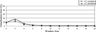$(K=1)$ .

Fig. 13

Classification error dependence on the number of neighbors, when both scattering parameters and their statistics were employed for discrimination.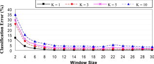

3.2.1.

Classification with spatial statistical data included

Figure 14 depicts the segmentation of one of the tumor samples into its distinct tumor regions in three different cases: employing only the scattering parameters (three-dimensional space), only their statistics (12-dimensional space) and both of them concatenated (15-dimensional space), while the corresponding confusion matrices are summarized in Table 3 . The improvement in the correlation between automated and expert-based sample segmentation within the regions of interest is barely perceptible. Sample boundary detection is significantly improved when statistics calculation is employed. Because when only the scattering parameters were considered, boundaries were improperly classified as mature fibrosis. The segmentation of the other four tumor samples in their distinct tumor regions is presented in Fig. 15 . These results are obtained employing a $12\text{-}\text{pixel}$ window size, concatenating the new calculated statistical parameters and the fitted scattering parameters, and their overall confusion matrix is presented in Table 4 . In this process, unclassified pixels were assigned to the same class as the closest one in the training set. Window sizes had to be as large as possible in such a way that the four statistical moments became relevant, but also small enough to assure that the moments are mostly computed for pixel localizations inside the same tissue subtype. A window size of $12\text{pixels}$ assured the latter in most situations because it implies a window side of $\sim 1.2\mathrm{mm}$ and, apart from that, classification error remains nearly constant for greater window sizes.²⁶

Fig. 14

Qualitative comparison among segmentations of one tumor sample in the distinct feature spaces are shown (scattering parameter feature space, statistical data, and both scattering parameters and their statistical values).

Fig. 15

Segmentation performance of some tumor samples are illustrated, employing a $12\text{-}\text{pixel}$ window size in statistical calculation, with a 15-dimensional feature space $(K=1)$ .

Table 3

Tumor sample number 2 confusion matrices in tumor subtype discrimination in the distinct feature spaces: (a), scattering parameter feature space (b) statistical data, and both scattering parameters and their statistical values.

	LPIepithelium	HPIepithelium	Necrosis	Earlyfibrosis	Intermediatefibrosis	Matiurefibrosis
LPI epithelium	279	0	0	0	0	0
HPI epithelium	0	187	0	0	0	0
Necrosis	0	0	183	0	0	0
Early fibrosis	5	0	0	269	0	0
Intermediate fibrosis	5	0	0	0	107	0
Mature fibrosis	0	0	0	0	0	0
(a) 3 variables
LPI epithelium	279	0	0	0	0	0
HPI epithelium	0	187	0	0	0	0
Necrosis	0	0	183	0	0	0
Early fibrosis	0	0	0	274	0	0
Intermediate fibrosis	0	0	0	0	112	0
Mature fibrosis	0	0	0	0	0	0
(b) 12 variables
LPI epithelium	279	0	0	0	0	0
HPI epithelium	0	187	0	0	0	0
Necrosis	0	0	183	0	0	0
Early fibrosis	0	0	0	274	0	0
Intermediate fibrosis	0	0	0	0	112	0
Mature fibrosis	0	0	0	0	0	0
(c) 15 variables

Table 4

Overall confusion matrix in tumor subtype discrimination in the 15-dimensional feature space (K=1) .

	LPIepithelium	HPIepithelium	Necrosis	Earlyfibrosis	Intermediatefibrosis	Maturefibrosis
LPI epithelium	1251	0	0	0	0	0
HPI epithelium	0	799	0	0	0	0
Necrosis	0	0	616	0	0	0
Early fibrosis	0	0	0	307	0	0
Intermediate fibrosis	0	0	0	0	459	0
Mature fibrosis	0	1	0	0	0	228

The subtype separability measurements through the SFFS algorithm, as described in Sec. 2, were computed for the 15 features, the scattering parameters, and their statistics. The first five features selected according to this criterion and as a function of the window size are summarized in Table 5, where $\overline{p}$ and ${\sigma }_p$ are, as indicated before, the mean and variance of the scattering parameter $p$ , and $K_p$ stands for its kurtosis moment. For smaller window sizes, which means that mostly vicinity regions will be within the same tissue subtype, the mean scattering power is always selected as the most discriminant feature.

Table 5

Sorting of the scattering parameters and their statistics as a function of their tissue subtype discrimination capability.

Window size	1	2	3	4	5
30	${\sigma }_A$	$\overline{A}$	$K_{I_{\mathrm{avg}}}$	$\overline{b}$	$\overline{I_{\mathrm{avg}}}$
28	${\sigma }_A$	$\overline{A}$	$K_{I_{\mathrm{avg}}}$	$\overline{I_{\mathrm{avg}}}$	$\overline{b}$
26	${\sigma }_A$	$\overline{A}$	$K_{I_{\mathrm{avg}}}$	$\overline{I_{\mathrm{avg}}}$	$\overline{b}$
24	${\sigma }_A$	$\overline{A}$	$K_{I_{\mathrm{avg}}}$	$\overline{I_{\mathrm{avg}}}$	$\overline{b}$
22	$K_b$	$K_{I_{\mathrm{avg}}}$	$\overline{I_{\mathrm{avg}}}$	${\sigma }_A$	$\overline{A}$
20	$K_b$	$K_{I_{\mathrm{avg}}}$	$\overline{I_{\mathrm{avg}}}$	$\overline{b}$	$\overline{A}$
18	$\overline{b}$	$\overline{I_{\mathrm{avg}}}$	$\overline{A}$	$K_b$	${\sigma }_A$
16	$\overline{b}$	$\overline{I_{\mathrm{avg}}}$	${\sigma }_{I_{\mathrm{avg}}}$	$\overline{A}$	$K_{I_{\mathrm{avg}}}$
14	$\overline{b}$	$\overline{I_{\mathrm{avg}}}$	${\sigma }_{I_{\mathrm{avg}}}$	$\overline{A}$	$K_{I_{\mathrm{avg}}}$
12	$\overline{b}$	$\overline{I_{\mathrm{avg}}}$	$\overline{A}$	$I_{\mathrm{avg}}$	${\sigma }_A$
10	$\overline{A}$	$\overline{I_{\mathrm{avg}}}$	$\overline{A}$	$I_{\mathrm{avg}}$	${\sigma }_A$
8	$\overline{b}$	$\overline{A}$	$\overline{I_{\mathrm{avg}}}$	${\sigma }_A$	$I_{\mathrm{avg}}$
6	$\overline{b}$	$\overline{A}$	$\overline{I_{\mathrm{avg}}}$	${\sigma }_A$	${\sigma }_{I_{\mathrm{avg}}}$
4	$\overline{b}$	$\overline{A}$	$\overline{I_{\mathrm{avg}}}$	${\sigma }_A$	$I_{\mathrm{avg}}$
2	$\overline{b}$	$\overline{A}$	$\overline{I_{\mathrm{avg}}}$	${\sigma }_A$	$I_{\mathrm{avg}}$