
|
|
1.IntroductionDiffuse optical tomography (DOT) can be used to image the optical properties of human tissue up to depths of several centimeters. Main clinical applications that are currently explored are breast imaging, functional brain imaging, and imaging of the neonatal brain.1 In typical DOT systems for breast imaging, near-infrared (NIR) laser light is radiated into the tissue successively from different source positions. The light propagates through the tissue and is affected by scattering and absorption. The intensity of the light emanating from the tissue is measured at a number of detector positions for each source position. From these measurements, three-dimensional (3-D) absorption and/or scattering images of the tissue can be reconstructed. The systems mainly differ in the geometry of source and detector positions, and in the light that is emitted into the tissue. While the geometry primarily affects the field of view and the local resolution and sensitivity in the images, the choice of the light sources has a major impact on what can be reconstructed from the measurements. There are two main aspects regarding the light sources. The first aspect is the variation of light intensity over time. Three schemes are common: short pulses ,2, 3, 4 modulated amplitude,5, 6 and continuous wave.7, 8, 9, 10 For a short light pulse, a time response of the light intensity can be measured at each detector position [time domain (TD) measurement]. For amplitude modulated light, amplitude and phase of the light intensity can be measured [frequency domain (FD) measurement]. For continuous wave light, only the steady-state amplitude of the light intensity can be measured [continuous wave (CW) measurement]. The different amount of information that is acquired for these three illumination schemes influences the reconstruction. While it is possible to separate scattering and absorption in reconstructions based on TD and FD measurements, this is not possible for CW measurements without a priori knowledge.11 The second aspect is the wavelength of the light. Most DOT systems successively use light with different wavelengths for the measurements (spectral measurement). How many and which wavelengths are used differs from system to system. Spectral measurements are useful, since absorption and scattering in tissue are wavelength dependent. The wavelength dependency of absorption is dominated by a few chromophores that mainly cause absorption in tissue (for breast: oxyhemoglobin, deoxyhemoglobin, water, and lipid). The chromophores have distinct wavelength dependencies in the relevant NIR band (see the following). Using these dependencies, the spatial distribution of the chromophore concentrations can be derived from the reconstructed absorption images for the different wavelengths,12, 13, 14, 15 if the wavelengths are chosen properly, i.e., quantitative values of physiological parameters of the tissue can be imaged, allowing us to determine physiological parameters such as blood volume and oxygenation. The wavelength dependency of the scattering is influenced by the effective size, the number density, and the index of refraction change of the scattering particles in tissue.16 It can be described in good approximation by a Mie scattering model: . The spatial distribution of the model parameters can be calculated based on the reconstructed scattering images for the different wavelengths.12, 13, 14, 15 Alternatively, using absorption spectra of the chromophores and a spectral model for the scattering, chromophore concentrations and scattering model parameters can be reconstructed directly from the spectral measurements (spectral reconstruction).9, 17, 18, 19, 20, 21 This spectral reconstruction leads to improved results,19 because the spectral dependency of absorption and scattering is used as a priori knowledge. Furthermore, spectral reconstruction works also for CW measurements.9, 18, 21 Prerequisites for a good estimation of chromophore concentrations and scattering parameters with spectral CW DOT systems are that the laser wavelengths are chosen properly and that the impact of deviations of a priori knowledge from reality is negligible. Corlu 21 describe a spectral reconstruction algorithm for spectral CW DOT systems. Moreover, they suggest an approach to determine an optimal set of wavelengths, by considering the separability of absorption and scattering and the separability of the chromophores. Thus, the method of Corlu meets one of the prerequisites stated earlier, and is consequently adequate, if the spectral models for scattering and chromophores are exactly known. If this is not the case, the uncertainties of the spectral models should be taken into account for the optimization of the wavelengths, to minimize reconstruction errors. This seems to be necessary especially for the chromophores, since the reported absorption spectra show significant differences (see the following). In this paper, an extension to the method given by Corlu is presented, which considers uncertainties in the chromophore absorption spectra. In Sec. 2, the basics of image reconstruction for optical tomography are introduced, and the incorporation of spectral models for scattering and absorption is explained. In Sec. 3, the method of Corlu for wavelength optimization and our extension are described. In Sec. 4, simulations are shown, which are done to analyze the effect of different wavelengths sets on reconstructed images. In Sec. 5, examples for wavelength sets determined with the new method are presented, and the effect of the choice of the wavelengths on the reconstruction is illustrated. In the last section, a conclusion is given. 2.Spectral ReconstructionThe propagation of NIR light in breast tissue is dominated by scattering. Thus, light propagation can be described by the diffusion equation,22 here given for the CW case: where is the photon density, is the diffusion coefficient (with being the reduced scattering coefficient), is the absorption coefficient, and is the speed of light in the turbid medium. models the light source. Note that photon density, absorption, and diffusion coefficient, as well as the light source function, are spatially varying functions, which additionally depend on the wavelength of the light.Furthermore, a boundary condition is necessary to describe the behavior of light at the boundaries of the imaging region. Commonly, a Robin-type boundary condition is applied:22 is the normal vector of the boundary surface, and is related to the mismatch of the refractive indices at the boundary.To come to a description that does not depend on absorption and diffusion coefficients, but on chromophore concentrations and parameters of the scattering model, the relationship between absorption coefficient and chromophore concentrations has to be known, as well as the relationship between reduced scattering coefficient and scattering model parameters. The relationship for the absorption coefficient is given by Beer’s law:18 is the molar absorption coefficient (derived from the absorption spectrum), and is the concentration of the ’th of chromophores.For the scattering coefficient, the relationship is given by a simplified Mie scattering model:16 The parameters of the model are the scattering amplitude and the scattering power . The normalization wavelength can be chosen arbitrarily.For the direct spatial reconstruction of chromophore concentrations and scattering parameters, and in Eqs. 3, 4 are substituted by the expressions given in Eqs. 1, 2. Then, the system given by Eqs. 1, 2 has to be solved for , , and , using the light intensities measured for the different wavelengths at the detector positions. This is a nonlinear, ill-posed inverse problem, which is commonly solved by iterative methods, with a linearization of the problem in each iteration step. A detailed description is given by Corlu 21 They found that it is difficult to reliably reconstruct both scattering parameters. For this reason, the scattering power will be set to a constant value in the following reconstructions, i.e., the scattering amplitude is the only scattering parameter that will be reconstructed. 3.Wavelength OptimizationIn addition to the reconstruction method, Corlu presented an algorithm to optimize the wavelengths of a spectral CW DOT system to optimally determine all parameters estimated by the reconstruction. The algorithm is based on two criteria, which are shortly described in the following. As stated earlier, CW DOT cannot distinguish scattering and absorption without a priori knowledge, because of the nonuniqueness of the solution of Eqs. 1, 2. Using spectral CW DOT and a spectral model for absorption and scattering, uniqueness is recovered, if the wavelengths are chosen properly. Thus, the first criterion evaluates whether the usage of a certain set of wavelengths leads to a unique solution for the chromophore concentrations and scattering parameters. The derivation is based on the nonuniqueness proof for CW measurements,11, 18 and leads to the expression are the wavelengths of the laser light used in the CW DOT system . The closer the residual norm is to zero, the closer the inverse problem is to nonuniqueness, i.e., the residual should be large for a proper set of wavelengths. Note that this automatically implies that the number of wavelengths has to be larger than the number of chromophores to achieve uniqueness of the inverse problem.The second criterion evaluates how well the chromophore concentrations can be distinguished. This can be directly derived from Beers law [see Eq. 3], if it is written in matrix form If the matrix with the molar absorption coefficients has a low condition number , all singular values are to some degree similar. This ensures that the measurements are roughly equally sensitive for all chromophores. Thus, a proper set of wavelengths should lead to a matrix with a low condition number.These two criteria depend, as expected, on the wavelengths of the lasers, on the scattering model, and on the molar absorption coefficients of the chromophores. The wavelengths of the lasers can be adjusted quite accurately. The scattering model appears to be consistent with real breast tissue in the relevant near-infrared band.23, 24 But the molar absorption coefficients given in literature for the main chromophores in breast tissue show significant deviations, as will be shown. For this reason, it is advantageous to choose a set of wavelengths that leads to a robust reconstruction of the chromophore concentrations, even if the assumed absorption spectra deviate from reality. In the following, a criterion is derived to allow for this. The starting point is Beer’s law 6. It is assumed that the matrix represents the assumed molar absorption coefficients. In the following, we furthermore introduce a matrix that contains the (unknown) correct molar absorption coefficients. The difference between these two matrices is defined as . According to Eq. 6, is the chromophore concentration vector, which gives the absorption vector after multiplication with . Analogously, we define as the concentration vector that gives if it is multiplied with . The difference between the two concentration vectors is . Thus, the equation holds for any given absorption vector . In other words: the error of the matrix results in an error of the concentration vector for a given absorption vector .To quantify this error, it is necessary to have an idea of , and to know the dependency of on and . Equation 7 can be solved for with a first-order approximation, if it is assumed that the entries of the matrix are small compared to the entries of : It should be noted that the absolute errors written in this form depend on . Since typical concentrations of the chromophores vary by several orders of magnitude, optimizing the absolute errors of is not meaningful. The interesting quantity are the relative errors of . To get these relative errors, we scale the entries of and with typical chromophore concentrations. Then, the vector becomes a vector of ones for the typical case, and contains the relative errors with respect to this case.If the standard deviations for the scaled molar absorption coefficients are known, they can be used to generate an assumption for the matrix and to calculate for a given set of wavelengths. Recapitulating, the norm of the errors is a measure for the reconstruction errors that can occur for the chromophore concentrations due to uncertainties in the absorption spectra of the chromophores. Thus, the new criterion is to choose a set of wavelengths with a small value for . All three introduced criteria [derived from the Eqs. 5, 6, 8] have to be considered simultaneously for an optimal set of wavelengths. For wavelength optimization, in the following, the scattering power is assumed to be 1, and typical values for the chromophore concentrations are assumed to be (oxygenated hemoglobin), (deoxygenated hemoglobin), and . These concentrations are used to scale the molar absorption coefficients for the calculation of . Furthermore, is also determined using the scaled molar absorption factors, to obtain more meaningful condition numbers. 4.Simulation and ReconstructionSimulated measurement data is used to verify the effect of the derived sets of wavelengths on the reconstruction result. This has the advantage that the values of molar absorption coefficients and of parameters of the scattering model are known exactly. Furthermore, the spatial distribution of chromophore concentrations and scattering values is also known and can be compared with the reconstruction result. In the following, we use a circular 2-D phantom with a diameter of . Five circular inhomogeneities with a diameter of are embedded in the background (see Fig. 1 ). The absorption in the background is caused by 50% water, 25% lipid, oxygenated hemoglobin and deoxygenated hemoglobin. The scattering follows the Mie scattering model, with a scattering amplitude and a scattering power . In four of the five inhomogeneities, one of the chromophore concentrations is increased by 5% with respect to the background. In the fifth inhomogeneity, the scattering amplitude is increased by 5%. The phantom is surrounded by 24 sources and 24 detectors, as can be seen in Fig. 1. Fig. 1The 2-D phantom used in the simulations is circular and has a diameter of . The concentrations of water , lipid , and deoxyhemoglobin and oxyhemoglobin ( and ) and values of the scattering parameters and in the phantom are given on the right. In four of the inhomogeneities, one of the chromophore concentrations is increased by 5% with respect to the background. In the fifth inhomogeneity, the scattering amplitude is increased by 5%. 24 sources and 24 detectors surround the phantom. 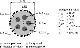 The measurement data is simulated by solving the Eqs. 1, 2 with finite element methods (FEM), using the deal.II library.25 The reconstruction is implemented using the methods described in Ref. 26. The nonlinear inverse problem is linearized, and the emerging linear system of equations is solved by direct inversion. The linearization uses a homogeneous object with the parameters of the background medium as a starting point.26 Since the optical properties of the inhomogeneities deviate only slightly from the background, this linearization is sufficient to lead directly to a reasonable result. To avoid image artifacts near sources and detectors,27 a spatially varying gradient regularization is used, in contrast to Ref. 26. A more sophisticated approach is given in Ref. 27. The chromophore absorption spectra and the scattering model can be chosen freely for simulations as well as for reconstruction. 5.ResultsDifferent absorption spectra are available for water,28, 29, 30, 31, 32 lipid,32, 33, 34, 35, 36 oxyhemoglobin, and deoxyhemoglobin.32, 37, 38 The spectra used here are presented in Fig. 2, showing significant deviations. Reasons for these deviations are, among others, that the optical properties of oxygenated and deoxygenated hemoglobin as well as human fat cannot be measured directly in vivo but have to be approximated by ex vivo measurements or measurements of similar substances (e.g., vegetable oil for human fat). The amount of deviation depends on the regarded chromophore and wavelength. To consider this chromophore and wavelength-dependent uncertainty, the standard deviations are determined and used as entries for the matrix in Eq. 8: where is the molar absorption coefficient of the ’th of absorption spectra for the ’th chromophore at the wavelength .Fig. 2Published absorption spectra for oxyhemoglobin, deoxyhemoglobin, water, and lipid show significant deviations.  For the calculation of the three criteria [derived from the Eqs. 5, 6, 8], the values of the molar absorption coefficients are set to the mean value of all available spectra: To find an optimal set of five wavelengths for the imaging of all four chromophores and the scattering amplitude, the three criteria are computed for all possible combinations of wavelengths between 650 and ( step size; approximately 120,000 combinations). The histograms of condition number, residual, and norm of errors are shown in part in Fig. 3 . As can be seen, many wavelength sets lead to a good condition and a low norm of the errors, but only a few lead to a high residual. From this visualization, it does not become clear, if there are wavelength sets, which lead to good values for all three criteria at the same time.Fig. 3Histograms of the three criteria for all possible wavelength combinations: Condition number (top); residual (middle); and norm of the errors (bottom). 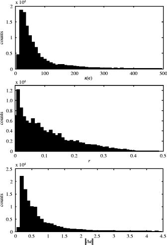 To come to a clearer visualization that illustrates the additional benefit of the new criterion, the two 2-D plots in Fig. 4 are used. Each dot in the plot on the left represents one set of wavelengths and its - and -values. In the plot on the right, the histogram of -values is plotted for all sets of wavelength, for which the values of and are within a narrow range, indicated by the dotted box in the left plot, i.e., considering only the two criteria based on and , all these sets of wavelengths perform comparably. But looking at the histogram, it can be seen that the distribution of the -values is quite wide. In other words, the performance of the sets with respect to uncertainties in the spectra varies a lot. Only those sets with a low value of are assumed to be optimal. Fig. 4Left: Plot of -values versus -values. Each point represents a set of five wavelengths. Right: Histogram of the -values for those sets with and (dotted rectangle in the left plot). 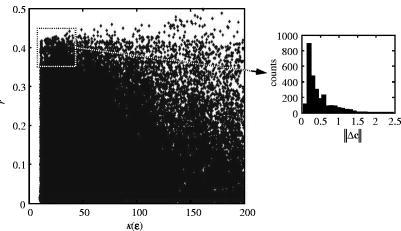 Since it is quite difficult to choose an optimal set from this kind of visualizations, a combined value of all three criteria is preferable. A simple weighted summation turned out to be a good solution. The weights are necessary, because the three criteria vary with different order of magnitude, as can be seen in Fig. 3. The combined value is calculated as follows: The factors were determined empirically using Fig. 3 and are somewhat arbitrary, but their exact values are not critical for the resulting sets of wavelengths.Figure 5 shows the 150 best sets of wavelengths (i.e., with the highest value of ). As could be expected, the sets are very similar. The first wavelength always has a value around (mean of the 150 best sets: ), the second around (mean: ), the third around (mean: ), the fourth around (mean: ), and the fifth around (mean ). To test whether these wavelengths result from the particular assumptions we made on the average tissue composition (50% water, 50% fat), we repeated the whole analysis for a tissue composition that is dominated by fat (70% fat, 30% water) and a tissue composition that is dominated by water (70% water, 30% fat). The resulting sets of wavelengths are only marginally different (mean for 70% water/30% fat: 653, 721, 810, 866, ; mean for 30% water/70% fat: 653, 718, 809, 863, ). Fig. 5Best 150 sets of wavelengths. Each column in the plot represents one set of five wavelengths. The first wavelength is marked with a circle, the second with a dot, the third with a diamond, the fourth with a star, and the fifth with a triangle. 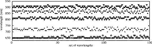 These sets of wavelength are different from those obtained without the third criterion, where the five preferred wavelengths have values around 650, 720, 870, 910, and (see Corlu 21). A probable reason for this discrepancy is the quite large deviations of the absorption spectra for water and lipid for wavelengths above (see Fig. 2). The values of , , and give an initial idea of the performance of a set of wavelengths. As an example, we analyze two sets in greater detail. The first set (650, 720, 810, 870, and ) is optimal if the norm of errors is ignored; the second set (650, 720, 870, 910, and ) is optimal if all three criteria are considered (see earlier). The -value, which is a measure for the separability of the chromophores, is 11.2 for the first set and 15.2 for the second set. This is a marginal change for the condition value of a matrix, i.e., the performance of the two sets with respect to the separability of the chromophores should be similar. The residual norm has a value of 0.39 for both sets; in other words, the uniqueness of the problem is equally assured for both sets. The -value is 0.58 for the first set and 0.15 for the second set. This means that the root mean square (RMS) of the relative errors for typical values of water, fat, and hemoglobin is reduced from 58% to 15%, which seems to be a quite significant reduction of the reconstruction errors due to deviations in the absorption spectra. To verify that the sets shown in Fig. 5 indeed minimize these reconstruction errors, simulated data for the phantom shown in Fig. 1 are reconstructed for the two sets of wavelengths. In the simulation we used, the mean absorption spectra according to Eq. 10 are applied. For the reconstruction, the spectral power is fixed to 1 (the same value as in the simulations). All combinations of the available water, fat, and hemoglobin spectra are applied successively, leading to 64 different reconstruction results (4 water spectra fat spectra hemoglobin spectra). Additionally, a reconstruction is performed using the mean absorption spectra (as in the simulations). For each combination of spectra, three scalar values benchmarking the image quality are determined, concerning the quantification of the chromophores, the cross talk between chromophores, and the artifacts in the images. These scalars are explained in detail in the following. To evaluate the quantification of the chromophores, in each image the RMS of the pixel values covering the inhomogeneity which is expected to give a signal in the respective image is determined (e.g., in the water image, the RMS of the pixel values covering the water inhomogeneity is determined). The difference between this RMS value and the expected value in the according inhomogeneity is divided by the expected value to derive a relative error. The absolute values of these relative errors are averaged over the five images of one reconstruction. The resulting scalar is called quantification error in the following: is the index running over all images , in our case, four chromophore images and the scattering amplitude image . is the set of all pixels covering inhomogeneity , and is the number of pixels in this set. The indexing is done such that the ’th inhomogeneity is expected to generate a signal in the ’th image. is the pixel value of the ’th pixel in the ’th image, and is the expected signal in the ’th inhomogeneity.To evaluate the cross talk of the chromophores, in each image the RMS values for all inhomogeneities that are expected to give no signal in the respective image are determined, divided by the expected signal in this image and averaged over all inhomogeneities and images of one reconstruction. The resulting scalar is called cross-talk error : To evaluate artifacts in the background, in each image the RMS for the background pixels is calculated and divided by the expected signal in this image. The RMS values are again averaged over all images, leading to the artifact error : is the set of all background pixels, and is the number of pixels in this set.In Fig. 6, these three benchmark values are shown for all 64 reconstruction for both sets of wavelengths. The quantification error (left) is comparable for both sets, while the crosstalk error is clearly reduced for the second set of wavelengths, showing the effectiveness of the new criterion for optimization. The artifact level (right) is also in average slightly better for the new set. Fig. 6Quantification error (left), cross-talk error (middle), and artifact error (right) for all 64 combinations of water, fat, and hemoglobin spectra. The dots represent the results for the first set of wavelengths (ignoring the norm of errors), the circles the results for the second set of wavelengths (considering the norm of errors). Cross talk is clearly reduced by the second set and artifacts are on average slightly reduced, while quantification errors are comparable. 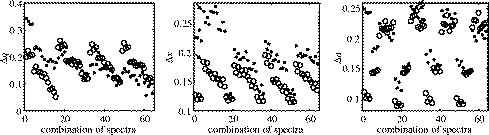 To get an idea how the reconstructed images look, three of the 64 reconstruction results are shown for each set of wavelengths:
The reconstruction results are presented in Fig. 7 for the first set of wavelengths. The top row shows the chromophore concentrations and scattering amplitude for the case in which the mean absorption spectra are used for reconstruction. Only weak image artifacts and cross talk are present, since the absorption spectra for simulation and reconstruction are identical. The images in the second row show severe imaging artifacts, especially for water. In the third row, the example with strong cross talk between the chromophores and scattering amplitude is given. The oxyhemoglobin image suffers from significant cross talk of water and scattering, the water image shows cross talk of scattering and deoxyhemoglobin, and the lipid image of water. Fig. 7Reconstruction results for simulated data at 650, 720, 870, 910, and . Top: Reconstruction with mean absorption spectra. Middle: Reconstruction showing strongest artifacts. Absorption spectra of Takatani (hemoglobin), Segelstein (water), and PTB (lipid). Bottom: Reconstruction showing strongest cross talk. Absorption spectra of Wray (hemoglobin), Kou (water), and van Veen (lipid). All images are scaled from 0.95 (black) to 1.05 (white) times the respective background value of the phantom (see Fig. 1).  These findings can now be compared to reconstruction results obtained with the second set of wavelengths (Fig. 8 ). Again, the top row shows the results for the case in which the mean absorption spectra are used for reconstruction. These images are largely comparable to those of Fig. 7. The artifacts at the rim of the water image are reduced. The images of the second row are reconstructed using the combination of absorption spectra leading to strong image artifacts. Compared to the corresponding images in Fig. 7, the artifacts are slightly reduced. The last row presents the images for the combination of absorption spectra that produces strong cross talk. But here cross talk is nearly not visible and significantly lower than for the first set of wavelengths. Fig. 8Reconstruction results for simulated data at 650, 720, 810, 870, and . Top: Reconstruction with mean absorption spectra. Middle: Reconstruction showing strongest artifacts (same absorption spectra as in Fig. 7). Bottom: Reconstruction showing strongest cross talk (same absorption spectra as in Fig. 7). The images are scaled the same way as in Fig. 7.  To verify that these results hold also if noisy data is used for reconstruction, different amounts of relative noise are added to the simulated measurement data before reconstruction. Relative noise up to 0.5% is applied, since for noise levels of 1% and higher, the artifact errors for both sets of wavelengths are above 90%, i.e., the inhomogeneities are completely buried by noise. To come to a compact presentation of the results, the benchmark values , , and are averaged over all 64 combinations of different spectra. The results are shown in Fig. 9 . Clearly, the advantage of reduced cross talk is still valid for noisy data (left plot), while artifacts and quantification errors (not shown) are comparable in the presence of noise. Fig. 9Cross-talk error (left) and artifact error (right) averaged for all 64 combinations of water, fat, and hemoglobin spectra for reconstructions with different amounts of relative noise. The dots represent the results for the first set of wavelengths (ignoring the norm of errors), the circles the results for the second set of wavelengths (considering the norm of errors). The advantage of reduced cross talk for the second set is also valid for noisy data. Artifacts and quantification errors (not shown here) are comparable for both sets in the presence of noise.  Recapitulating the findings, we conclude that the introduced new criterion for wavelength optimization leads clearly to the intended minimization of cross talk, while artifacts and quantification errors are comparable to sets of wavelengths optimized without that criterion. 6.ConclusionThe introduced method for the optimization of laser wavelengths for CW DOT systems considers, in contrast to existing methods, the uncertainties in the absorption spectra of the chromophores. The absorption spectra are essential for reconstruction, if absorption and scattering should be distinguishable in CW DOT. For each of the chromophores, four absorption spectra were compared, revealing significant deviations. Considering these deviations led to optimal sets of wavelengths different from those determined ignoring the uncertainties in the absorption spectra. It was demonstrated with simulated data that reconstructions based on the new sets of wavelength are significantly more robust with respect to cross talk, if the assumed absorption spectra deviate from reality. Recently, Eames published a method, also based on the criteria of Corlu, to optimize sets with a much larger number of wavelengths than considered here.20 It is straightforward to include the criterion introduced here in this method. Last, it should be noted that although this discussion is focused on CW data, it is straightforward to apply the introduced method to TD of FD measurements. AcknowledgmentsThe authors would like to express their gratitude to Albert Cerussi (University of Irvine, California), Alper Corlu (University of Pennsylvania, Philadelphia), and Dirk Grosenick (Physikalisch-Technische Bundesanstalt, Berlin, Germany) for providing chromophore absorption spectra. ReferencesA. P. Gibson, J. C. Hebden, and S. R. Arridge,
“Recent advances in diffuse optical imaging,”
Phys. Med. Biol., 50 R1
–R43
(2005). https://doi.org/10.1088/0031-9155/50/4/R01 0031-9155 Google Scholar
S. R. Arridge and M. Schweiger,
“A finite element approach for modeling photon transport in tissue,”
Med. Phys., 20 299
–309
(1993). https://doi.org/10.1118/1.597069 0094-2405 Google Scholar
M. Schweiger and S. R. Arridge,
“Application of temporal filters to time resolved data in optical tomography,”
Phys. Med. Biol., 44 1699
–1717
(1999). https://doi.org/10.1088/0031-9155/44/7/310 0031-9155 Google Scholar
D. Grosenick, H. Wabnitz, H. Rinneberg, K. T. Moesta, and P. M. Schlag,
“Development of a time-domain optical mammograph and first in vivo applications,”
Appl. Opt., 38 2927
–2943
(1999). https://doi.org/10.1364/AO.38.002927 0003-6935 Google Scholar
N. Shah, A. Cerussi, C. Eker, J. Espinoza, J. Butler, J. Fishkin, R. Hornung, and B. Tromberg,
“Noninvasive functional optical spectroscopy of human breast tissue,”
Proc. Natl. Acad. Sci. U.S.A., 98 4420
–4425
(2001). https://doi.org/10.1073/pnas.071511098 0027-8424 Google Scholar
B. W. Pogue, S. Geimer, T. O. McBride, S. Jiang, U. L. Osterberg, and K. D. Paulsen,
“Three-dimensional simulation of near-infrared diffusion in tissue: boundary condition and geometry for finite-element image reconstruction,”
Appl. Opt., 40 588
–600
(2001). https://doi.org/10.1364/AO.40.000588 0003-6935 Google Scholar
S. B. Colak, M. B. van der Mark, W. ’t Hooft, J. H. Hoogenraad, E. S. van der Linden, and F. A. Kuijpers,
“Clinical optical tomography and NIR spectroscopy for breast cancer detection,”
IEEE J. Sel. Top. Quantum Electron., 5 1143
–1158
(1999). https://doi.org/10.1109/2944.796341 1077-260X Google Scholar
T. Nielsen, B. Brendel, R. Ziegler, F. Uhlemann, C. Bontus, and T. Koehler,
“Linear image reconstruction for a diffuse optical mammography system in a non-compressed geometry using scattering fluid,”
Appl. Opt., 48 D1
–D13
(2009). https://doi.org/10.1364/AO.48.0000D1 0003-6935 Google Scholar
A. Li, Q. Zhang, J. P. Culver, E. L. Miller and D. A. Boas,
“Reconstructing chromosphere concentration images directly by continuous-wave diffuse optical tomography,”
Opt. Lett., 29 256
–258
(2004). https://doi.org/10.1364/OL.29.000256 0146-9592 Google Scholar
K. Lee, R. Choe, A. Corlu, S. D. Konecky, T. Durduran, A. G. Yodh,
“Artifact reduction in CW transmission diffuse optical tomography,”
(2004) Google Scholar
S. R. Arridge and W. R. B. Lionheart,
“Nonuniqueness in diffusion-based optical tomography,”
Opt. Lett., 23 882
–884
(1998). https://doi.org/10.1364/OL.23.000882 0146-9592 Google Scholar
B. W. Pogue, S. Jiang, H. Deghani, C. Kogel, S. Soho, S. Srinivasan, X. Song, T. D. Tosteson, S. P. Poplack, and K. D. Paulsen,
“Characterization of hemoglobin, water, and NIR scattering in breast tissue: analysis of intersubject variability and menstrual cycle changes,”
J. Biomed. Opt., 9 541
–552
(2004). https://doi.org/10.1117/1.1691028 1083-3668 Google Scholar
A. E. Cerussi, D. Jakubowski, N. Shah, F. Bevilacqua, R. Lanning, A. J. Berger, D. Hsian, J. Butler, R. F. Holcombe, and B. J. Tromberg,
“Spectroscopy enhances the information content of optical mammography,”
J. Biomed. Opt., 7 60
–71
(2002). https://doi.org/10.1117/1.1427050 1083-3668 Google Scholar
T. Durduran, R. Choe, J. P. Culver, L. Zubkov, M. J. Holboke, J. Giammarco, B. Chance, and A. G. Yodh,
“Bulk optical properties of healthy female breast tissue,”
Phys. Med. Biol., 47 2847
–2861
(2002). https://doi.org/10.1088/0031-9155/47/16/302 0031-9155 Google Scholar
A. Pifferi, J. Swartling, E. Chikoidze, A. Torricelli, P. Taroni, and A. Bassi,
“Spectroscopic time-resolved diffuse reflectance and transmittance measurements of the female breast at different interfiber distances,”
J. Biomed. Opt., 9 1143
–1151
(2004). https://doi.org/10.1117/1.1802171 1083-3668 Google Scholar
X. Wang, B. W. Pogue, S. Jiang, X. Song, K. D. Paulsen, C. Kogel, S. P. Poplack, and W. A. Wells,
“Approximation of Mie scattering parameters in near-infrared tomography of normal breast tissue in vivo,”
J. Biomed. Opt., 10 051704
(2005). https://doi.org/10.1117/1.2098607 1083-3668 Google Scholar
S. Srinivasan, B. W. Pogue, S. Jiang, H. Dehghani, and K. D. Paulsen,
“Spectrally constrained chromophore and scattering near-infrared tomography provides quantitative and robust reconstruction,”
Opt. Express, 14 5394
–5410
(2006). https://doi.org/10.1364/OE.14.005394 1094-4087 Google Scholar
A. Corlu, T. Durduran, R. Choe, M. Schweiger, E. M. C. Hillman, S. R. Arridge, and A. G. Yodh,
“Uniqueness and wavelength optimization in continuous-wave multispectral diffuse optical tomography,”
Opt. Lett., 28 2339
–2341
(2003). https://doi.org/10.1364/OL.28.002339 0146-9592 Google Scholar
B. Brooksby, S. Srinivasan, S. Jiang, H. Deghani, B. W. Pogue, K. D. Paulsen, J. Weaver, C. Kogel, and S. P. Poplack,
“Spectral priors improve near-infrared diffuse tomography more than spatial priors,”
Opt. Lett., 30 1968
–1970
(2005). https://doi.org/10.1364/OL.30.001968 0146-9592 Google Scholar
M. E. Eames, J. Wang, B. W. Pogue, and H. Deghani,
“Wavelength band optimization in spectra near-infrared optical tomography improves accuracy while reducing data acquisition and computational burden,”
J. Biomed. Opt., 13 054037-1
–054037-9
(2008). https://doi.org/10.1117/1.2976425 1083-3668 Google Scholar
A. Corlu, R. Choe, T. Durduran, K. Lee, M. Schweiger, S. R. Arridge, E. M. C. Hillman, and A. G. Yodh,
“Diffuse optical tomography with spectral constraints and wavelength optimization,”
Appl. Opt., 44 2082
–2093
(2005). https://doi.org/10.1364/AO.44.002082 0003-6935 Google Scholar
S. R. Arridge,
“Optical tomography in medical imaging,”
Inverse Probl., 15 R41
–R93
(1999). https://doi.org/10.1088/0266-5611/15/2/022 0266-5611 Google Scholar
A. E. Cerussi, A. J. Berger, F. Bevilacqua, N. Shah, D. Jakubowski, J. Butler, R. F. Holcombe, and B. J. Tromberg,
“Sources of absorption and scattering contrast for near-infrared optical mammography,”
Acad. Radiol., 8 211
–218
(2001). https://doi.org/10.1016/S1076-6332(03)80529-9 1076-6332 Google Scholar
F. Bevilacqua, A. J. Berger, A. E. Cerussi, D. Jakubowski, and B. J. Tromberg,
“Broadband absorption spectroscopy in turbid media by combined frequency-domain and steady-state methods,”
Appl. Opt., 39 6498
–6507
(2000). https://doi.org/10.1364/AO.39.006498 0003-6935 Google Scholar
W. Bangerth, R. Hartmann, and G. Kanschat,
“deal.II—a general-purpose object-oriented finite element library,”
ACM Trans. Math. Softw., 33 1
–27
(2007). https://doi.org/10.1145/1268776.1268779 0098-3500 Google Scholar
B. Brendel, R. Ziegler, and T. Nielsen,
“Algebraic reconstruction techniques for spectral reconstruction in diffuse optical tomography,”
Appl. Opt., 47 6392
–6403
(2009). https://doi.org/10.1364/AO.47.006392 0003-6935 Google Scholar
M. E. Eames and H. Deghani,
“Wavelength dependence of sensitivity in spectral diffuse optical imaging: effect of normalization on image reconstruction,”
Opt. Express, 16 17780
–17791
(2008). https://doi.org/10.1364/OE.16.017780 1094-4087 Google Scholar
G. M. Hale and M. R. Querry,
“Optical constants of water in the to wavelength region,”
Appl. Opt., 12 555
–563
(1973). https://doi.org/10.1364/AO.12.000555 0003-6935 Google Scholar
M. R. Querry, P. G. Cary, and R. C. Waring,
“Split-pulse laser method for measuring attenuation coefficients of transparent liquids: application to deionized filtered water in the visible region (E),”
Appl. Opt., 17 3587
–3592
(1978). https://doi.org/10.1364/AO.17.003587 0003-6935 Google Scholar
L. Kou, D. Labrie, and P. Chylek,
“Refractive indices of water and ice in the 0.65- to 2.5-m spectral range,”
Appl. Opt., 32 3531
–3540
(1993). https://doi.org/10.1364/AO.32.003531 0003-6935 Google Scholar
D. J. Segelstein,
“The complex refractive index of water,”
Univ. of Missouri–Kansas City,
(1981). Google Scholar
S. Prahl,
“Tabulated molar extinction coefficient for hemoglobin in water,”
(1999) Google Scholar
C. Eker,
“Optical characterization of tissue for medical diagnostics,”
Lund University,
(1999). Google Scholar
R. L. P. van Veen, H. J. C. M. Sterenborg, A. Pifferi, A. Torricelli, and R. Cubeddu,
“Determination of VIS-NIR absorption coefficients of mammalian fat, with time- and spatially resolved diffuse reflectance and transmission spectroscopy,”
Proc. Biomedical Topical Meetings,
(2004) Google Scholar
V. Quaresima, S. J. Matcher, and M. Ferrari,
“Identification and quantification of intrinsic optical contrast for near-infrared mammography,”
Photochem. Photobiol., 67 4
–14
(1998). https://doi.org/10.1111/j.1751-1097.1998.tb05159.x 0031-8655 Google Scholar
D. Grosenick,
“Lipid absorption spectrum measured by the Physikalisch-Technische Bundesanstalt (PTB), Berlin, Germany,”
Google Scholar
M. K. Moaveni,
“A multiple scattering field theory applied to whole blood,”
(1970) Google Scholar
S. Takatani and M. D. Graham,
“Theoretical analysis of diffuse reflectance from a two-layer tissue model,”
IEEE Trans. Biomed. Eng., 26 656
–664
(1979). https://doi.org/10.1109/TBME.1979.326455 0018-9294 Google Scholar
|


